L6 Systematic Trading Strategies and Systems

Systematic Trading

• systematic trading uses data (primarily price and volume) to discover patterns, test whether they endure, control risk continuously and execute with discipline and consistency

What is Systematic Trading

• rule based trading or mechanical trading
  • auto (machines) / algotrading
  • semi-auto (human and machines)
  • manual (humans)
• rules → variables → parameters
  • you don’t trade stocks, you trade rules
• backtest
  • risk management
• elimination of emotions
  • after all, it’s humans who trade
  • decisions are driven by desires - greed and fear
  • traditional models → behavioural finance → social finance

Backtesting

• simulate a trading rule on historical data to evaluate how it would have performed

Backtesting Steps

• get historical data
• simulate your trading in historical data
  • identify the signals
  • record buy / sell points
  • calculate the PNL and other metrics
• fit variations on historical period and finalise the best model
• assumes historical patterns may persist; good past performance does not guarantee future results
• different ways to backtest

Backtesting Types

• in sample backtest
  • choose the best variation using all N years, then report performance on those same years
  • results can look too good due to overfitting; earlier years are evaluated using a rule selected with later data
• out of sample backtest
  • split chronologically into an earlier training (in sample) period and a later test (out of sample) period
  • optimise and select the variation on training data, then evaluate it on unseen test data
  • holds back data from training; a fixed model does not adapt to market changes during testing
• expanding window
  • fit on all available past data, then test on the next period (e.g. 1 year)
  • add that period to training, refit and test on the following period; the training window grows
  • e.g. train years 1–3 → test 4; train 1–4 → test 5
• rolling window
  • use a fixed-length training window; move it forward, dropping the oldest data, then refit and test
  • e.g. train years 1–3 → test 4; train 2–4 → test 5
  • focuses on recent market conditions, but uses less training data
• expanding and rolling windows are walk-forward testing: each test period uses only earlier data for fitting

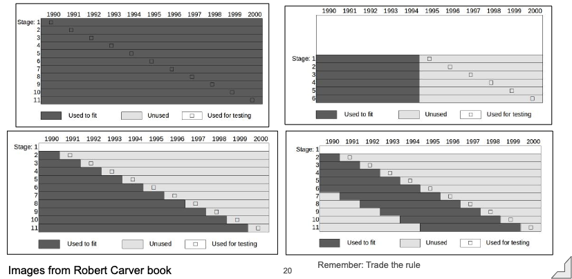
• legend: columns = years; rows = test stages; dark grey = fitting data; square = test period; light grey = unused for fitting
• top left: in sample: fit on all years, then test those same years; includes future data relative to earlier tests
• top right: out of sample: fit once on 1990–1994, then test later years without refitting
• bottom left: expanding: refit using all past data before each test; training window grows
• bottom right: rolling: once the window reaches its fixed length, move it forward and drop the oldest data before refitting

Variations in Backtesting

• variation: a different parameter setting for a trading rule, e.g. different moving-average lengths
• with hundreds of variations, options include choosing the best, choosing randomly, or combining variations with equal / unequal weights
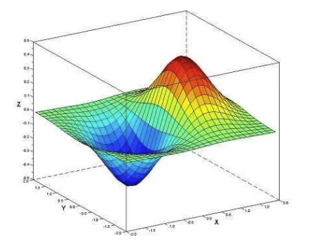
• the best historical result may reflect luck rather than a better rule; testing more variations increases the chance of finding a misleading winner (overfitting)
• another naive approach: select variations with similar performance in training and test periods, then combine them
  • if test results influence selection, that period is no longer an independent test; evaluate the final choice on fresh unseen data

How much data is needed?

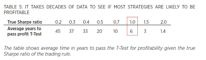
• to trust in sharpe ratio, how much data is needed?
• experiment: generated returns for a positive sharpe. keep on measuring the SR as the new data comes and then measure the distribution and mean
• 2 sigma test. if estimated SR > 2 sigma, only a 2.5% chance of being negative
• t-test for profitability
  

Best Practices

• small number of rules
• few variations. look at returns, if highly correlated, drop the variations
• select variations that show similar result in both train and test periods individually
• assign weights to each variation
  • equal weights or optimised weights or bootstrapped weights
• for midterm, single variation will be ok

Vectorised vs Event Based Backtesting

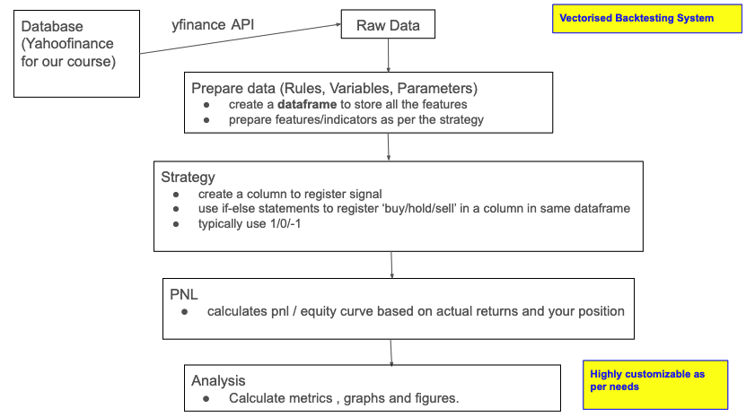
• Vectorised Backtesting
  • computationally efficient and easy to implement
  • focuses on signal generation and deals with overall returns
  • uses daily returns to evaluate signal profitability
  • no explicit modelling of trade execution (no quantities, transaction fees, leverage etc)
  • calculations performed using dataframes
• Event-Based Backtesting
  • more realistic simulation of trading strategies
  • explicitly models trade execution and portfolio dynamics
  • tracks profits and losses, cash balances and position sizes
  • incorporates risk management and money management rules
  • calculations using loops and advanced coding techniques
    

MA Cross in python

1. Install and import libraries
2. Create initial helper variables like dates and symbols for backtesting
3. Check if the data is OK
4. Define the RULES
5. Visualise if signals exists
6. Create dataframe to store data and perform vectorised backtesting
7. Create a column “Position” based on your Rule
8. Create a column “Strategy Returns “ based on ‘Position’ and ‘Stock returns’.
9. Calculate Mean, Standard deviation and Sharpe Ratio
   • on both Stock and Strategy column

Notebook code snippets

• rule → variables → parameters: compare fast / slow moving averages, using 5 / 21 trading days

import numpy as np
 
bt_data = hist_stock[["Close"]].rename(columns={"Close": "Close_Price"}).copy()
bt_data["STMA"] = bt_data["Close_Price"].rolling(5).mean()
bt_data["LTMA"] = bt_data["Close_Price"].rolling(21).mean()
bt_data = bt_data.dropna()
 
bt_data["Position"] = np.where(bt_data["STMA"] > bt_data["LTMA"], 1.0, -1.0)
bt_data["Signal"] = bt_data["Position"].diff()

• rolling().mean() is equivalent to the notebook’s SMAIndicator; drop the initial rows without enough history
• Position: +1 = long, −1 = short; this rule assigns −1 when the averages are equal too
• Signal: +2 = short → long, −2 = long → short, 0 = unchanged; position is the holding, signal marks a change

bt_data["Stock_Returns"] = np.log(
    bt_data["Close_Price"] / bt_data["Close_Price"].shift(1)
)
bt_data["Strategy_Returns"] = (
    bt_data["Stock_Returns"] * bt_data["Position"].shift(1)
)
returns = bt_data[["Stock_Returns", "Strategy_Returns"]].dropna()
growth = np.exp(returns.cumsum())
total_return = np.exp(returns.sum()) - 1

• shift(1) is essential: today’s close determines today’s position, which earns the next period’s return; using today’s position on today’s return introduces look-ahead bias
• follows the notebook’s simplified execution at the signal close, without costs; multiplying log returns by −1 is an approximation for short-position returns
• log returns add over time; exp(cumsum()) gives growth of 1 unit, while exp(sum()) - 1 gives total return
• annualisation: daily mean × 252; daily standard deviation × √252. The notebook’s Sharpe calculation assumes a zero risk-free rate and uses an annual return converted from log returns

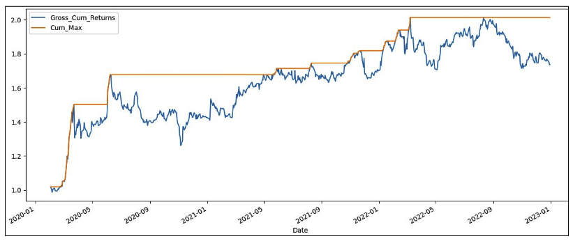
Drawdown

equity = growth["Strategy_Returns"]
peak = equity.cummax().clip(lower=1.0)  # include initial wealth of 1
drawdown = peak - equity
max_drawdown = drawdown.max()

• cummax() tracks the highest value reached so far; drawdown is the fall below that peak
• the notebook measures an absolute gap in wealth units; percentage drawdown is 1 - equity / peak
• its longest drawdown calculation uses gaps between peak dates; it misses an unrecovered drawdown at the end