L3A Risk and Returns

Stock Returns

• Daily Returns: $(P_t-P_{t-1})/P_{t-1}$
  • aka. simple / regular / norm
• Log Returns: $\ln (P_t/P_{t-1})$
  • additive → takes into account compounding effect
• Absolute Returns: $(P_{last}-P_{first})/P_{first}$
• Expected Returns: $E[R]={\sum }_i{P}_i{R}_i$, or mean of returns
  • $P_i$ = probability of state $i$ (weights, ${\sum }_i{P}_i=1$); $R_i$ = return in that state
  • ⚠️ notation clash: this $P$ is not the price $P_t$ from the bullets above — subscript shifts $t\to i$
  • equal probabilities $P_i=1/n$ → collapses to the plain arithmetic mean (the historical case, returns.mean())
  • same shape for portfolios, with allocation weights $w_i$ in place of $P_i$: $R_p={\sum }_i{w}_i{R}_i$

$$\begin{array}{c}E[R]=\sum _{i=1}^n{P}_i{R}_i\\ P_i=\frac{1}{n}⟹E[R]=\frac{1}{n}\sum _{i=1}^n{R}_i=\bar{R}\end{array}$$ $$\begin{array}{c}Log\_R=\ln (1+\text{Regular\_R})\\ \text{Regular\_R}=\exp (Log\_R)-1\end{array}$$

Why log returns (an example)

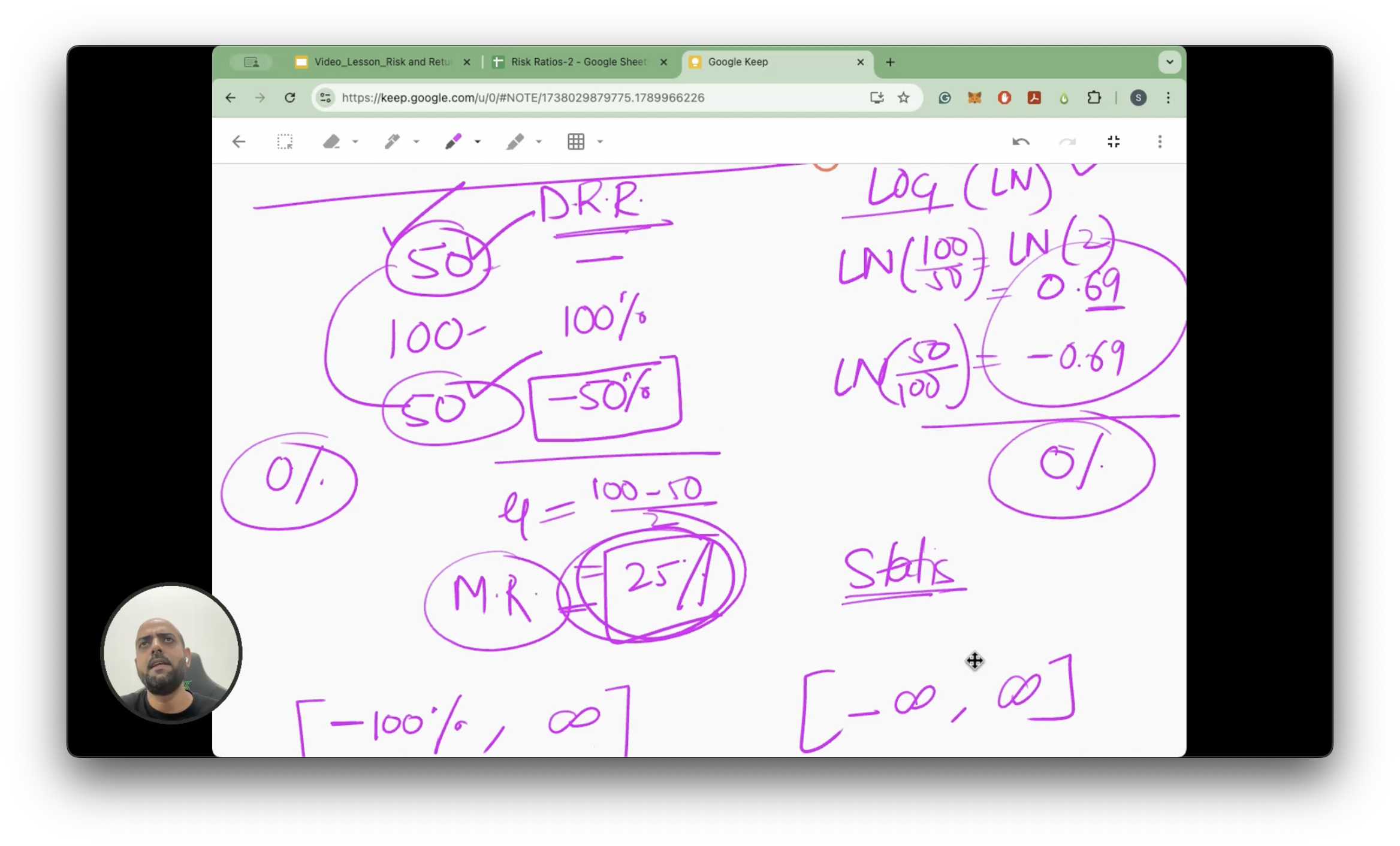
Deliberately extreme numbers, to expose what breaks when you average regular returns.

Day	Price	Regular return	Log return
0	$50	—	—
1	$100	$(100-50)/50=+100\%$	$\ln (100/50)=\ln 2=+0.693$
2	$50	$(50-100)/100=-50\%$	$\ln (50/100)=-\ln 2=-0.693$
		$\mu =\frac{100+(-50)}{2}=+25\%$	$\mu =\frac{0.693+(-0.693)}{2}=0$

• the stock opened at $50 and closed at $50 → in reality you gained 0%
  • but the mean of the regular returns claims +25% per day — a gain that exists nowhere
  • the mean of the log returns gives 0 ✅ → matches what actually happened
• cause: regular returns are multiplicative across time, so they don’t average meaningfully
  • $\ln$ converts the multiplicative chain into an additive one → the sum of log returns is the total log return: ${\sum }_t\ln (P_t/P_{t-1})=\ln (P_{last}/P_{first})=\ln (50/50)=0$
  • strictly: the arithmetic mean of regular returns is not “wrong”, it’s just not the compound growth rate - it answers a different question
• second problem with regular returns - asymmetric bounds
  • downside floored at $-100\%$ (a stock can at worst go to 0)
  • upside unbounded, can run to $+\infty$
  • → distribution is skewed, not normal, which breaks any stats that assume normality
  • log returns are unbounded in both directions, range $(-\infty ,+\infty )$ → far better behaved
• ⇒ use log returns for statistical work, or whenever regular returns aren’t normally distributed

when the price changes are small, log ≈ regular, so the distinction stops mattering much in practice. the gap only blows up on extreme moves like this 100% / -50% example

Histogram of Returns

• using excel / python or any tool
• histogram plots out the counts / frequency of particular ranges of values
• from the histogram shown:
  
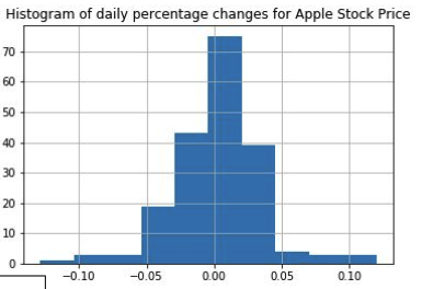
  • most of the days’ percentage changes are around 0
  • very few days have more than 10% changes in the stock price (in either direction)
• not the individual values, but the behaviour matters

Standard Deviation (~Risk)

• dispersion relative to mean
• high SD, higher the volatility
• Volatility ~ Risk

$$\sigma =\sqrt{\frac{\sum (x_i-\mu {)}^2}{N}}$$

• ${\sigma }^2=\text{Variance}$

Normal Distribution

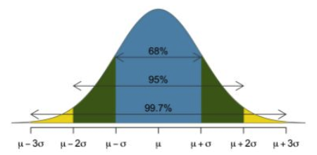
• in general:
  • about 95% of values will fall within 2 standard deviations from the mean
  • about 99.7% of values will fall within 3 standard deviations from the mean

Projections

• for normal distributions with given mean and std deviation

$$\begin{array}{c}68\%\text{ confidence}\to \mu +\sigma ,\mu -\sigma \\ 95\%\text{ confidence}\to \mu +2\sigma ,\mu -2\sigma \\ 99.7\%\text{ confidence}\to \mu +3\sigma ,\mu -3\sigma \end{array}$$

Scaling to N days

• daily data gives ${\mu }_d,{\sigma }_d$ → convert before projecting over N days

$$\begin{array}{c}{\mu }_N=N\times {\mu }_d\\ {\sigma }_N=\sqrt{N}\times {\sigma }_d\end{array}$$

• $\sigma$ does not extrapolate linearly: variance adds across days ($N{\sigma }_d^2$), and $\sigma$ is its square root → $\sqrt{N}$
• eg. price 100, ${\mu }_d=0.2\%$, ${\sigma }_d=1.2\%$, 68% band over 5 days:
  • ${\mu }_5=5(0.2\%)=1\%$, ${\sigma }_5=\sqrt{5}(1.2\%)=2.68\%$
  • ${\mu }_5\pm {\sigma }_5$ → $1\%\pm 2.68\%$ → $-1.68\%$ to $+3.68\%$ → price 98.32 to 103.68

Closing notes

• annualising: $N=252$ trading days/yr for equities (weekends removed), but $N=365$ for crypto (traded every day)
• compute in log space, report in regular space — a $50 stock going to $100 made 100%, you don’t report 69.2%; convert back with $\exp (Log\_R)-1$
  • small returns → can just assume normality, log ≈ regular; only drastic moves need the log detour
• risk = deviation you did not expect — even when it moves in your favour
• these $\mu ,\sigma$ projections are what real trading platforms use to forecast (alongside time-series analysis)