L4 Trading Strategies and Systems

Reading Charts

time based
- each point/candle represents a fixed time interval
- line charts
- candlesticks
price based
- new entries require sufficient price movement; equal spacing does not mean equal elapsed time
- point and figure (box size and reversal count)
- many others (Renko, Kagi, etc.)

Line and Candlesticks

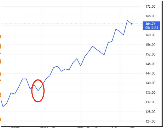
Line Chart
- only close prices
- makes the overall trend easy to see, but hides price swings within each interval
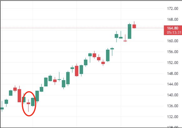
Candlesticks
- Open-High-Low-Close (OHLC)
- body = open to close; wicks extend to the interval’s high and low
- close above open = rising candle; close below open = falling candle
- depends on intervals / frequency - 5M, 15M, 1D etc.
- mostly this data through API’s

Point and Figure

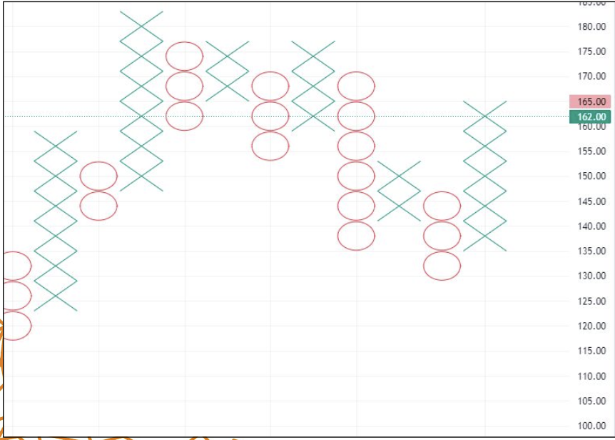
built from closing prices; ATR (Average True Range) can set box size based on volatility
X column = rising prices; O column = falling prices
box size = 2: each X/O represents a $2 move; smaller moves are ignored
reversal = 6: needs a 6-box ($12) opposite move to start a new column
time alone does not create a new entry—only price movement does
TA principles still apply: trends, support/resistance and breakouts
filters market noise → fewer false breakouts, but later signals

Renko and Kagi

Renko - bricks of a chosen price size
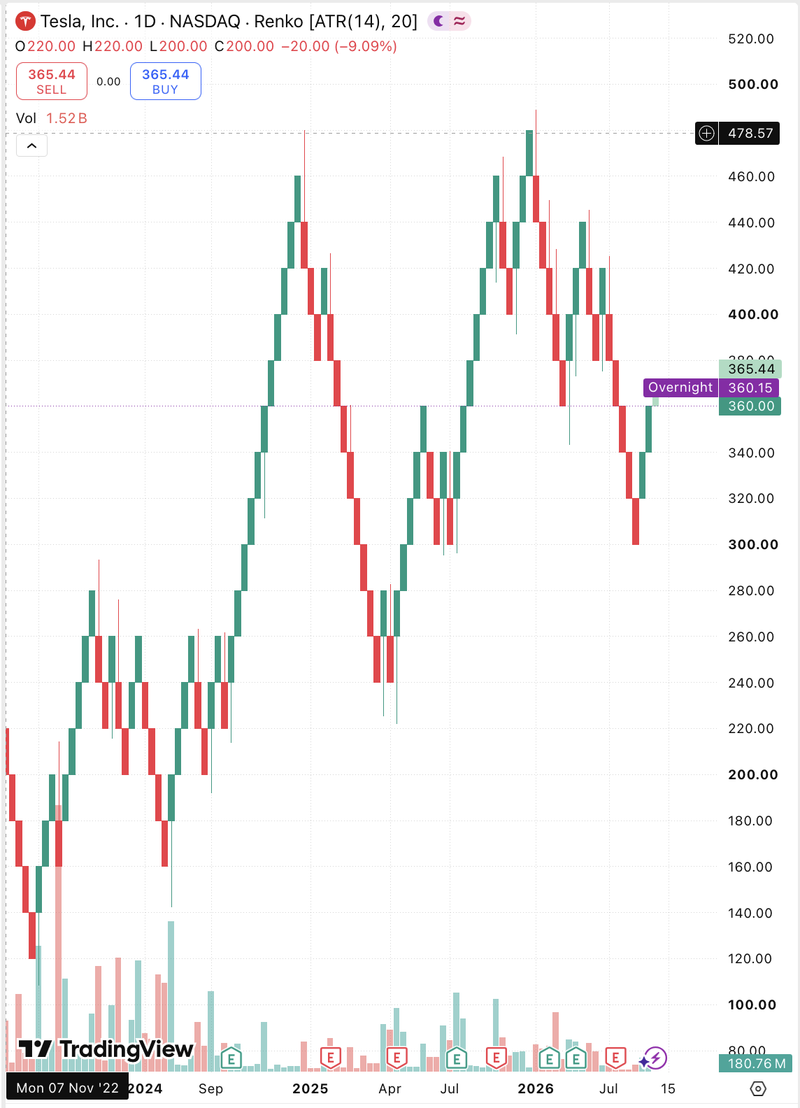
- adds bricks when price crosses the required thresholds; small moves produce no new brick
- example with $2 b r i c k s : a f t er an u pw a r d b r i c k f ro m$ 100 to $102, t h e n e x t u pw a r d b r i c k re q u i res$ 104; a reversal brick requires $98 (a tw o - b r i c k d ro p f ro m$ 102)
- brick size can be fixed or based on ATR; larger bricks filter more noise but delay signals
- useful for seeing trends and support/resistance. Reference: TradingView
Kagi - connected vertical lines with a reversal threshold
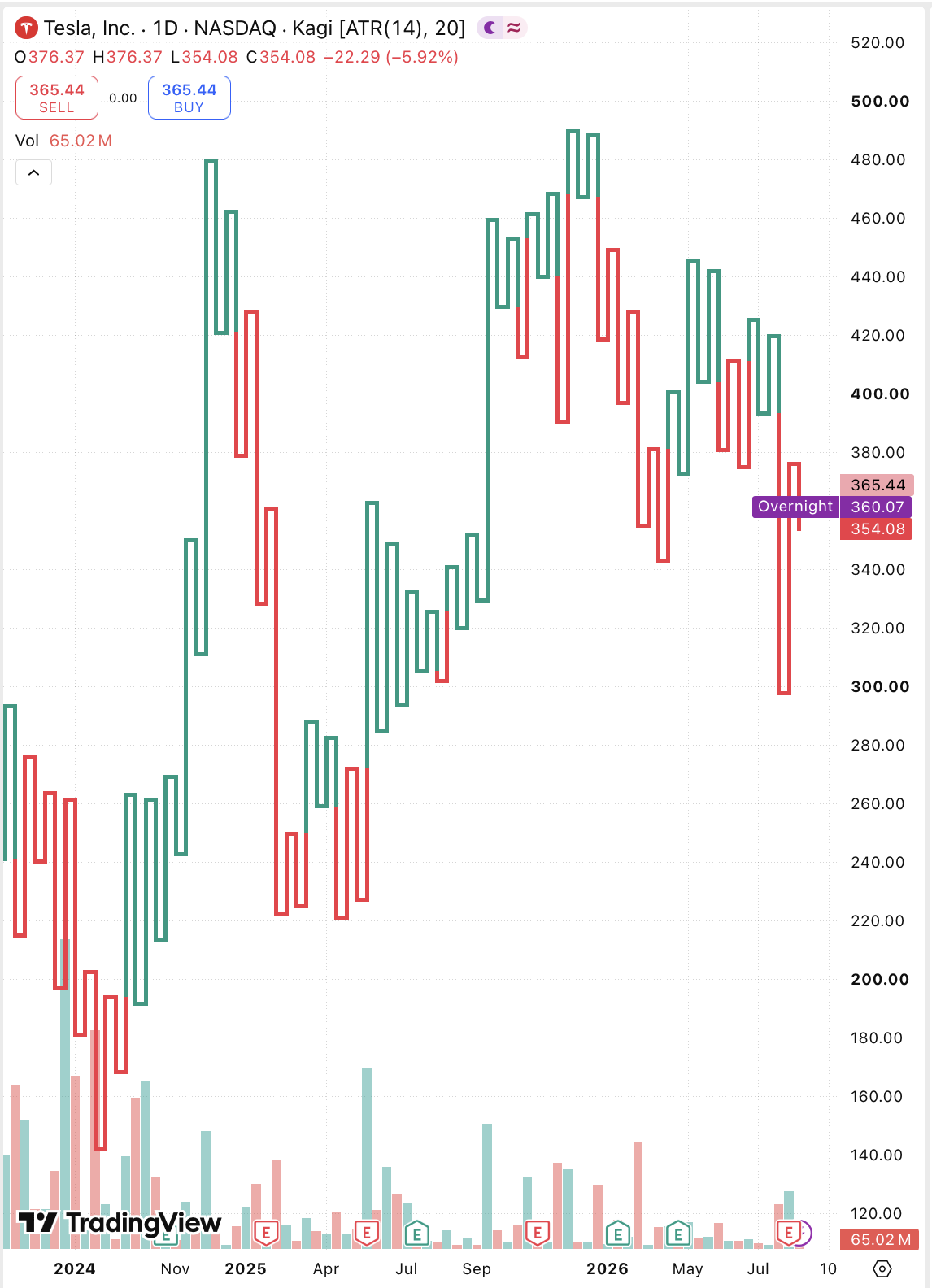
- extends the current line while price continues in the same direction; changes direction only after an opposite move reaches the chosen reversal amount
- example with a $2 re v ers a l : i f an u pw a r d l in ere a c h es$ 105, a fall to $104 i s i g n ore d; a f a llt o$ 103 starts a new downward line, joined by a short horizontal line
- filters small fluctuations to highlight larger swings and support/resistance. Reference: TradingView

Use chart types together: candlesticks show timing and OHLC detail, while price-based charts help reveal the broader trend.

Vectorised Backtesting System

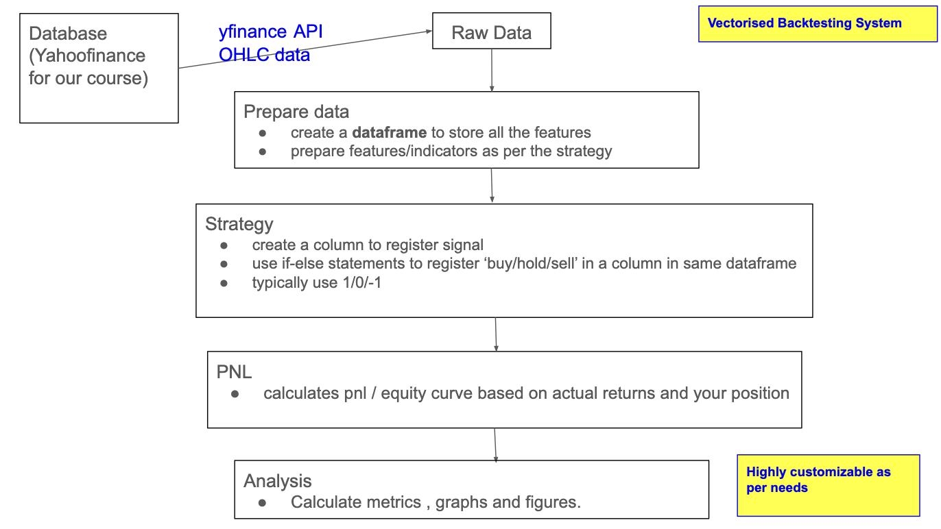
API’s

connects two systems / programs, bundled in libraries
- Yahoofinance
- Google FInance
- Quandl
- Alphavantage
- pandas datareader

Notebook Screenshots

Code below follows the notebook versions (including their dates), grouped to match the slides.

Setup and stock selection

# Use ! to install libraries..Some are by default
!pip install yfinance
 
import yfinance as yf
# yfinance an open source library. Thanks to Ran Aroussi. However, yahoo finance only for educational purposes. Dont download data
# https://pypi.org/project/yfinance/
# valid periods: 1d,5d,1mo,3mo,6mo,1y,2y,5y,10y,ytd,max
# valid intervals: 1m,2m,5m,15m,30m,60m,90m,1h,1d,5d,1wk,1mo,3mo. Intraday only for 60 days
 
import math
import pandas as pd
import numpy as np

# You can find the symbols in yahoofinance
# example for DBS https://sg.finance.yahoo.com/quote/D05.SI/
 
stock_symbol = "D05.SI"
benchmark_symbol = "^STI"
start="2024-01-01"
end="2024-08-31"
period = "1y" #period for starting today to past 1y

Stock information and historical prices

# Create a ticker object
stock_data = yf.Ticker(stock_symbol)
 
stock_data.info
 
#get historical data for a period
# Its real time
hist_stock = stock_data.history(period)
 
#get historical data from a start date to end date
hist_stock = stock_data.history(start=start,end=end)
 
#Plot only close
hist_stock["Close"].plot()

Benchmark and multiple tickers

#benchmark check
benchmark_data = yf.Ticker(benchmark_symbol)
hist_benchmark = benchmark_data.history(start=start,end=end)
hist_benchmark["Close"].plot()

#getting multiple stock data
mult_symbols = [benchmark_symbol, stock_symbol]
multiple_data = yf.Tickers(mult_symbols)
multiple_data

A = multiple_data.tickers["D05.SI"].history(period)["Close"]
A.plot()
 
B = multiple_data.tickers["^STI"].history(period)["Close"]
B.plot()

BASS Notebook Screenshots

Select stock and benchmark

# You can find the symbols in yahoofinance
# example for DBS https://sg.finance.yahoo.com/quote/D05.SI/
 
#"D05.SI" "^STI"
stock_symbol = "AAPL"
benchmark_symbol = "^GSPC"
start="2025-01-01"
end="2025-08-31"
period = "1y"

Prepare prices and returns

#BASS Calculation
 
#Prepare data with returns. Assumption is normal returns
df = pd.DataFrame()
df["benchmark"] = yf.Ticker(benchmark_symbol).history(start=start,end=end).Close
df["stock"] = yf.Ticker(stock_symbol).history(start=start,end=end).Close
df['benchmark_returns'] = df["benchmark"].pct_change()  #for now working with regular returns
df['stock_returns'] = df["stock"].pct_change()
df = df.dropna()
df.head()

Beta

#calculate Beta
cov = df['benchmark_returns'].cov(df['stock_returns'])
var = df['benchmark_returns'].var()
beta = cov/var
beta = round(beta,2)
print(beta)

#Another way to calculate Beta. Make a returns covariance matrix
returns = df[['stock_returns', 'benchmark_returns']]
#make a cov matrix
matrix = returns.cov()
# Select the variance and covariance to calculate beta.
beta = matrix.iat[1,0] / matrix.iat[1,1]
print("The beta is {:.2f}".format(beta))

Alpha and standard deviation

#calculate Alpha
#Can be calcultaed using annualised returns or Using absolute yearly returns.
#If more than a years data, you can use CAGR. Thats ((Final Price / Initial Price) ^ (1/t)) - 1
#assuming Risk free rate  as 0
 
benchmark_yearly_returns = (df["benchmark_returns"].mean()*252)
stock_yearly_returns = (df["stock_returns"].mean()*252)
alpha = (stock_yearly_returns - beta * benchmark_yearly_returns)*100
alpha = round(alpha,2)
print(alpha)

#calculate Standard deviation of stock
std_dev = (df['stock_returns'].std()) *100
std_dev = round(std_dev,2)
print(std_dev)

Alpha is annualised and expressed as a percentage, assuming a zero risk-free rate. Standard deviation here is daily, expressed as a percentage.

Sharpe ratio

#calculate Sharpe Ratio of stock
#SR = Mu/Sigma
# Remember that Sharpe is only for a stock. It has nothing to do with Markets.
# Used for comparing two stocks/portfolios
 
avg_returns = df['stock_returns'].mean()
std = df['stock_returns'].std()
daily_SR = avg_returns / std
#Convert daily to annual
annual_SR = daily_SR * (252**0.5)
annual_SR = round(annual_SR,2)
print(annual_SR)

This calculation also assumes a zero risk-free rate and uses 252 trading days to annualise the daily Sharpe ratio.

BASS function and stock list

#BASS as a function but here I am using a start date and end date
#Note that if you use a period of less than a year, then use annual returns accordingly.
 
def BASS(stock_symbol,benchmark_symbol,start,end):
 
  #Prepare data with returns. Assumption is normal returns
  df = pd.DataFrame()
  df["benchmark"] = yf.Ticker(benchmark_symbol).history(start=start,end=end).Close
  df["stock"] = yf.Ticker(stock_symbol).history(start=start,end=end).Close
  df['benchmark_returns'] = df["benchmark"].pct_change(fill_method=None)
  df['stock_returns'] = df["stock"].pct_change(fill_method=None)
  df = df.dropna()
 
 
  #calculate Beta
  cov = df['benchmark_returns'].cov(df['stock_returns'])
  var = df['benchmark_returns'].var()
  beta = cov/var
  beta = round(beta,2)
 
  #calculate Alpha
  benchmark_abs_returns = df["benchmark_returns"].mean()*252
  stock_abs_returns = df["stock_returns"].mean()*252
  alpha = (stock_abs_returns - beta * benchmark_abs_returns)*100
  alpha = round(alpha,2)
 
  #calculate Standard deviation of stock
  std_dev = (df['stock_returns'].std()) *100
  std_dev = round(std_dev,2)
 
  #calculate Sharpe Ratio of stock
  avg_returns = df['stock_returns'].mean()
  std = df['stock_returns'].std()
  daily_SR = avg_returns / std
  annual_SR = daily_SR * (252**0.5)
  annual_SR = round(annual_SR,2)
 
  return beta, alpha, std_dev, annual_SR

#List of all major singapore stocks
 
all_stocks = ["C52.SI", "S68.SI", "G13.SI", "V03.SI" , "U11.SI", "C07.SI" , "D05.SI", "Z74.SI",\
        "D01.SI", "O39.SI", "S63.SI", "A17U.SI" , "BN4.SI","BS6.SI", "M44U.SI", "H78.SI", \
        "Y92.SI", "C38U.SI", "U14.SI", "N2IU.SI" , "F34.SI" , "C09.SI" ,\
        "J36.SI", "S58.SI" , "C6L.SI", "U96.SI" ,\
        "1810.HK", "9999.HK", "7500.HK", "9618.HK", "1024.HK", "3690.HK", "6618.HK"]

Calculate and rank the stocks

#Create list to store values
stock_name =[]
beta_value =[]
alpha_value =[]
std_dev_value =[]
sharpe_value = []
 
benchmark_symbol = "^STI"
start="2024-01-01"
end="2024-08-31"
 
#Loop through all the stocks to calculate BASS
#Using try and except to pass the exceptions in case no data available and run the code for all stocks.
 
for i in all_stocks:
  try:
    BASS_output = BASS(i,benchmark_symbol,start,end)
    beta_value.append(BASS_output[0])
    alpha_value.append(BASS_output[1])
    std_dev_value.append(BASS_output[2])
    sharpe_value.append(BASS_output[3])
    stock_name.append(i)
  except:
    print('The symbol {} not found'.format(i))
 
# Prepare a dataframe from the above lists.
output_df = pd.DataFrame()
output_df['stock'] = stock_name
output_df['beta'] = beta_value
output_df['alpha(%)'] = alpha_value
output_df['standard_dev(%)'] = std_dev_value
output_df['sharpe'] = sharpe_value
 
 
# print the stocks with ascending Sharpe
print (output_df.sort_values(by="sharpe", ascending = False))

ascending=False sorts Sharpe ratios from highest to lowest; the notebook’s “ascending Sharpe” comment is a typo.

Trading Strategies

passive (static) or active (dynamic)
idea first or data first
trend following or mean reversion
sharpe and skew of the returns (positive or negative)
sharpe (5/5 or 1/1) and leverage to increase profit (risk vs reward)
fast (seconds to intraday) or slow (days to months)
technical (price action) or fundamental (micro to macro data)

Passive vs Active

Passive (Static)
- buy and hold approach, minimal security selection or strategy selection
- example: index funds, ETFs tracking S&P500
- objective: simply capture market returns without frequent adjustments
Active (Dynamic)
- involves frequent decision-making and trading
- example: hedge funds, discretionary traders, quant funds
- objective: beat the markets. outperform benchmarks or exploit inefficiencies

Idea First or Data First

Idea First : Deductive
- starts with a hypothesis, intuition or theory
  - example: momentum exists because of investor herding
  - before weekends / lunch break activities
  - the first hour of trading
- data is used later to test / validate the idea
Data First : Inductive
- starts with mining patterns or signals in large datasets
  - machine learning, extensive quant research
- idea or theory may come afterward to explain why the pattern works

Fast vs Slow

Fast
- seconds to minutes
- high-frequency trading, scalping, intraday strategies
- relies on microstructure, speed, excecution edge
Slow
- hours to days to months
- intraday, swing trades, position trades, macro bets
- relies on broader economic, fundamental, or trend signals

Positive or Negative Skew

negative skew:
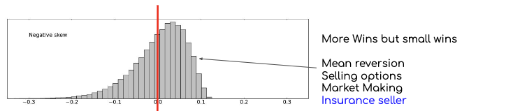
- more wins but small wins
positive skew:
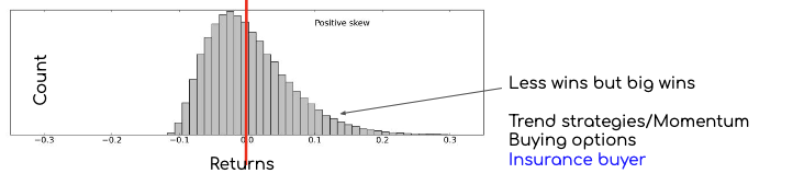
- less wins but big wins

Mean Reversion or Momentum

mean reversion
- asset prices return to their long term average
momentum
- continued rate of change of prices in same direction

Other Popular Strategies

pairs trading
- disturbed correlation between pairs
arbitrage
- inefficiencies in markets
market making
- spread betting
candlesticks patterns
- trading sentiment

kienans garden *

Explorer