L10 Simulation

Introduction

The objective of any simulation study is to estimate an expectation E(X). Simulation studies involve the use of a computer to generate independent copies of the random variable of interest X. Here are a couple of examples where simulation studies would be applicable.

Example 10.1 (Insurance Claims)

Before the financial year begins, an insurance company has to decide how much cash to keep, in order to pay out the claims for that year.

Suppose that claims are independent of each other and are distributed as $Exp(1/200)$ dollars. Also suppose that the number of claims in a year is s Poisson random variable with mean 8.2.

An actuary has been asked to determine the size of the reserve fund that should be set up, and he recommends $12,000. We might consider answering the following question using simulation:

• What is the probability that the total claims will exceed the reserve fund?

If we let Y be the random variable representing the total sum of claims, we are interested in estimating $P(Y>12000)$ . Since probabilities are expectations, we can use simulation to estimate this value.

Example 10.2 (Sandwich Shop Closing Time)

Suppose that you run a sandwich shop, which is open from 9am till 5pm. Your philosophy has always been to serve every customer who has entered before 5pm, even if that requires you to stay back until they have been served. You
would like to estimate the mean amount of overtime you have to work.

If you are willing to assume that the inter-arrival times of customers is 𝐸𝑥𝑝(3) hours, then it is possible to simulate this process to estimate the mean time that you would have to remain open, beyond 5pm.

:LiLightbulb: The two examples above are known as Discrete Event Simulations.
But in this course, we will just try to understand and familiarise ourselves with the basic building blocks of simulation studies.

The basic steps in a simulation study are:

1. Identify the random variable of interest and write a program to simulate it
2. Generate an iid sample $X_1,X_2,\dots ,X_n$ using this program.
3. Estimate $E(X)$ using $\bar{X}$
   This is sometimes referred to as Monte Carlo Simulation.

Theory

There are two important theorems that simulation studies rely on.

Theorem 10.1 - Strong Law of Large Numbers (SLLN)

If $X_1,X_2,\dots ,X_n$ are independent and identically distributed with $E(X)<\infty$ , then

$$\bar{X}=\frac{1}{n}\sum _{i=1}^n{X}_i\to E(X)\text{ with probability 1.}$$

In the simulation context, it means that as we generate more samples (ie. increase n), our sample mean $\bar{X}$ converges to the desired value E(X), no matter what the distribution of X is.

Theorem 10.2 - Central Limit Theorem (CLT)

Let $X_1,X_2,\dots ,X_n$ be i.i.d., and suppose that

• $-\infty <E(X_1)=\mu <\infty$.
• $\mathrm{Var}(X_1)={\sigma }^2<\infty$.
  Then

$$\frac{\sqrt{n}(\bar{X}-\mu )}{\sigma }\Rightarrow N(0,1)$$

where $\Rightarrow$ denotes convergence in distribution.
This is sometimes informally interpreted to mean that when $n$ is large, $\bar{X}$ is approximately Normal with mean $\mu$ and variance ${\sigma }^2/n$. In the simulation context, we can use this theorem to obtain a confidence interval for the expectation that we are estimating.

Also take note of the following properties of the sample mean and variance:

Theorem 10.3 (Sample Estimates)

It can be shown that both the sample mean and sample standard deviation are unbiased estimators.

$$E(\bar{X})=E(X),E(s^2)={\sigma }^2$$

where $s^2=\frac{\sum (X_i-\bar{X}{)}^2}{n-1}$

To obtain a $(1-\alpha )100$ confidence interval for $\mu$, we use the following formula, from the CLT:

$$\bar{X}\pm z_{1-\alpha /2}\frac{s}{\sqrt{n}}$$

When our goal is to estimate the probability of an event $A$, we have to introduce a corresponding indicator variable $X$ such that

$$X=\{\begin{array}{ll}1& \text{when }A\text{ occurs}\\ 0& \text{when }{A}^c\text{ occurs}\end{array}$$

In this case, the formula for the CI becomes

$$\bar{X}\pm z_{1-\alpha /2}\sqrt{\frac{\bar{X}(1-\bar{X})}{n}}$$

Generating Random Variables in R and Python

Both R and Python contain built-in routines for generating random variables from common “named” distributions, e.g. Normal, Uniform, Gamma, etc. All software that can generate random variables utilise Pseudo-Random Number Generators (PRNG). These are routines that generate sequences of deterministic numbers with very very long cycles. However, since they pass several tests of randomness, they can be treated as truly random variables for all intents
and purposes.

In both software, we can set the “seed”. This initialises the random number generator. When we reset the seed, we can reproduce the stream of random variables exactly. This feature exists:

1. For debugging purposes,
2. To allow us to study the sensitivity of our results to the seed.

Example 10.3 (Random Variable Generation)

R code

In R, all the functions for generating random variables begin with r (for random). Here are a few such functions:

$$\begin{array}{ll}\text{Function name}& \text{Random Variable}\\ \text{rnorm}& \text{Normal}\\ \text{runif}& \text{Uniform}\\ \text{rgamma}& \text{Gamma}\\ \text{rpois}& \text{Poisson}\\ \text{rbinom}& \text{Binomial}\end{array}$$

set.seed(2137)
 
opar <- par(mfrow=c(1,3))
Y <- rgamma(50, 2, 3)
hist(Y)
 
W <- rpois(50, 1.3) # 50 obs from Pois(1.3)
barplot(table(W))
 
Z <- rbinom(50, size=2, 0.3) # 50 obs from Binom(2, 0.3)
barplot(table(Z))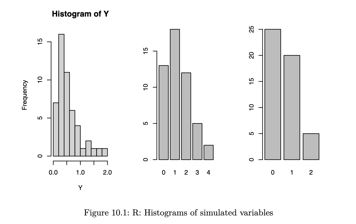

par(opar)

Python code

In Python, we can generate random variables using numpy and/or scipy. In our course, we shall use the scipy routines because its implementation is closer in spirit to R.

$$\begin{array}{ll}\text{Function name}& \text{Random Variable}\\ \text{norm}& \text{Normal}\\ \text{uniform}& \text{Uniform}\\ \text{gamma}& \text{Gamma}\\ \text{poisson}& \text{Poisson}\\ \text{binom}& \text{Binomial}\end{array}$$

import numpy as np
import pandas as pd
from scipy.stats import binom, gamma, norm, poisson
from scipy import stats
import matplotlib.pyplot as plt
 
rng = np.random.default_rng(2137)
fig, ax = plt.subplots(1, 3, figsize=(8,4))
 
ax1 = plt.subplot(131)
r = gamma.rvs(2, 3, size=50, random_state=rng)
ax1.hist(r);
 
ax1 = plt.subplot(132)
r = poisson.rvs(1.3, size=50, random_state=rng)
ax1.hist(r);
 
ax1 = plt.subplot(133)
r = binom.rvs(2, 0.3, size=50, random_state=rng)
ax1.hist(r);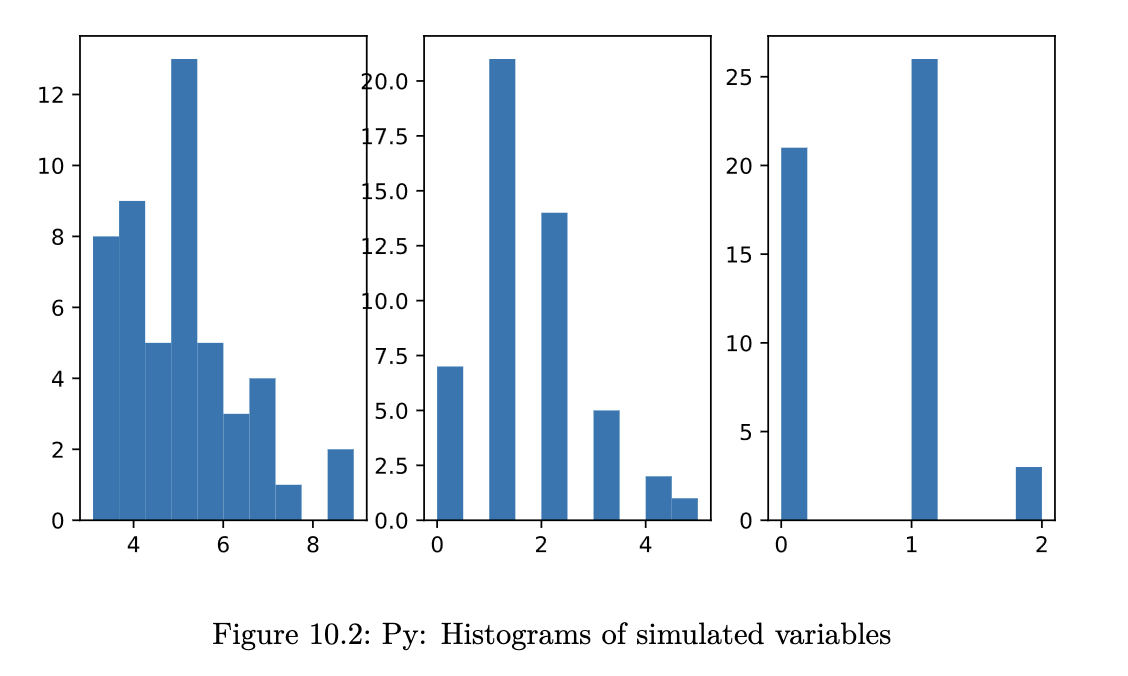

Monte-Carlo Integration

Suppose we wish to evaluate

$${\int }_{-\infty }^{\infty }h(x)f(x)dx$$

where f(x) is a pdf. The integral above is in fact to equal to $E(h(X))$ where $X\sim f$. Hence we can use everything we have discussed so far, to evaluate the expression using simulation.
Everything depends on:

1. Being able to introduce a pdf to the integral
2. Being able to simulate from that pdf

! Important
It is critical that the support of the pdf is the same as the range of integration.

Example 10.4 (Monte Carlo Integration over (0,1))

Suppose we wish to evaluate

$$\theta ={\int }_0^1{e}^{2x}dx={\int }_0^1{e}^{2x}\cdot 1dx$$

We can identify that this is equal to $E(h(X))$ where

• $X\sim \text{Unif}(0,1)$.
• $h(X)=e^{2x}$
  Thus we can follow this pseudo-code:

1. Generate $X_1,X_2,\dots ,X_n\sim \text{Unif}(0,1)$.
2. Estimate the integral using

$$\frac{1}{n}\sum _{i=1}^n{e}^{2X_i}$$

In this simple case, we can in fact work out analytically that the integral is equal to

$$\frac{1}{2}(e^2-1)=3.195$$

R code

set.seed(2138)
X <- runif(50000, 0, 1)
hX <- exp(2*X)
(mc_est <- mean(hX))
 
# [1] 3.185626

Python code

from scipy.stats import uniform
 
X = uniform.rvs(0,1, size=50000, random_state=rng)
hX = np.exp(2*X)
hX.mean()
 
# np.float64(3.2090955591090906)

Simulation Studies

In this section, we shall touch on how we can use simulation in some scenarios that are closer to the real world.

Confidence Intervals

The usual 95% confidence interval for a mean is given by

$$\bar{X}\pm t_{0.025}\frac{s}{\sqrt{n}}$$

where $t_{0.025}$ is the 0.025 quantile of the $t$-distribution with $n-1$ degrees. The resulting interval should contain the true mean in 95% of the experiments. However, it is derived under the assumption that the data is Normally distributed. Let us see if it still works if the data is from an asymmetric distribution: $\text{Pois}(0.5)$.

Example 10.5 (Coverage of Confidence Interval)

R code

set.seed(2139)
output_vec <- rep(0, length=100)
n <- 20
lambda <- 0.5
for(i in 1:length(output_vec)) {
  X <- rpois(n, .5)
  Xbar <- mean(X)
  s <- sd(X)
  t <- qt(0.975, n-1)
  CI <- c(Xbar - t*s/sqrt(n), Xbar + t*s/sqrt(n))
  if(CI[1] < lambda & CI[2] > lambda) {
    output_vec[i] <- 1
  }
}
mean(output_vec)
 
# [1] 0.92

Python code

rng = np.random.default_rng(2137)
output_vec = np.zeros(100)
n = 20
lambda_ = 0.5
for i in range(100):
    X = poisson.rvs(0.5, size=n, random_state=rng)
    Xbar = X.mean()
    s = X.std()
    t = norm.ppf(0.975)
    CI = [Xbar - t*s/np.sqrt(n), Xbar + t*s/np.sqrt(n)]
    if CI[0] < lambda_ and CI[1] > lambda_:
        output_vec[i] = 1
output_vec.mean()
 
# np.float64(0.86)

Type I Error

Consider the independent two-sample t-test that we introduced in L7 Two-sample Hypothesis Tests. The formal set-up also includes the assumption that our data arises from a Normal Distribution. According to the theory of the t-test, if both groups have the same mean, we could falsely reject the null hypothesis 10% of the time if we perform it at 10% significance level. Let us assess if this is what actually happens:

Example 10.6 (T-test Type I Error)

R code

generate_one_test <- function(n=100) {
  X <- rnorm(n)
  Y <- rnorm(n)
  t_test <- t.test(X, Y,var.equal = TRUE)
  # extract the p-value from the t_test
  if(t_test$p.value < 0.10) 
    return(1L) 
  else 
    return(0L)
}
 
set.seed(11)
output_vec <- vapply(1:2000, 
                     function(x) generate_one_test(), 
                     1L)
mean(output_vec)
 
# [1] 0.108

Python code

rng = np.random.default_rng(2137)
def generate_one_test(n=100):
    X = norm.rvs(0, 1, size=n, random_state=rng)
    Y = norm.rvs(0, 1, size=n, random_state=rng)
    t_test = stats.ttest_ind(X, Y, equal_var=True)
    if t_test.pvalue < 0.10:
        return 1
    else:
        return 0
output_vec = np.array([generate_one_test() for j in range(2000)])
output_vec.mean()
 
# np.float64(0.0975)

Newspaper Inventory

Example 10.7

Suppose that daily demand for newspaper is approximately gamma distributed, with mean 10,000 and variance 1,000,000. The newspaper prints and distributes 11,000 copies each day. The profit on each newspaper sold is $1,andthelossoneachunsoldnewspaperis\mathrm{0.25.}Formally,thedailyprofitfunction$h$ is

$$h(X)=\{\begin{array}{ll}11000& \text{if }X\ge 11000\\ \lfloor X\rfloor +(11000-\lfloor X\rfloor )(-0.25)& \text{if }X<11000\end{array}$$

where $X$ represents the daily demand. Let us estimate the expected daily profit using simulation.

R code

set.seed(2141)
n <- 10000
X <- rgamma(n, 100, rate=1/100)
hX <- ifelse(X >= 11000, 11000, floor(X) + (11000 - floor(X)) * (-0.25))
#mean(hX)
 
# 90% CI for the mean
s <- sd(hX)
q1 <- qnorm(0.95)
CI <- c(mean(hX) - q1*s/sqrt(n), mean(hX) + q1*s/sqrt(n))
cat("The 90% CI for the mean is (", format(CI[1], digits=2, nsmall=2), ", ", 
    format(CI[2], digits=2, nsmall=2), ").\n", sep="")
 
# The 90% CI for the mean is (9639.10, 9673.69).

Python code

n = 10000
X = gamma.rvs(100, scale=100, size=n, random_state=rng)
hX = np.where(X >= 11000, 11000, np.floor(X) + (11000 - np.floor(X)) * (-0.25))
 
# 90% CI for the mean
Xbar = hX.mean()
s = hX.std()
t = norm.ppf(0.95)
CI = [Xbar - t*s/np.sqrt(n), Xbar + t*s/np.sqrt(n)]
print(f"The 90% CI for the mean is ({CI[0]: .3f}, {CI[1]: .3f}).")
 
# The 90% CI for the mean is ( 9615.583, 9650.393).

Resampling Methods

This section introduces two techniques that are based on resampling data.

Permutation Test

Consider the two-sample t-test that we introduced in L7 Two-sample Hypothesis Tests. This parametric test requires us to check if the data from the two groups came from Normal distributions. The non-parametric version requires each group to have at least 10 observations. What if our data satisfies neither criteria?

The permutation test is applicable in such a situation. It makes no distributional assumptions whatsoever on the data. Here is the pseudo-code for how it works:

1. Compute the difference in group means. This observed difference is the test statistic
2. Treating the observed values as fixed, combine the two vectors of observations
3. Permute the observations, and then re-assign them to the two groups
4. Compute the difference between the group means
5. Repeat steps 2-4 multiples times (order of 1000)

The p-value for the null hypothesis can be computed by computing the proportion of simulated statistics that were larger in absolute value than the observed one.

Example 10.8 (Abalone Data)

See Example 7.1 (Abalone Measurements) for the output from the t-test.

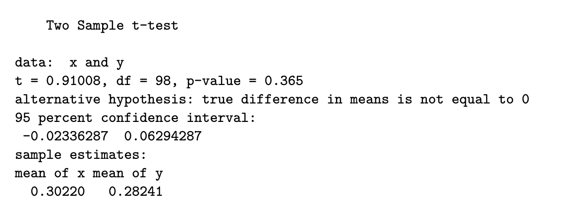
This would be the procedure for a permutation test:

d1 <- mean(x) - mean(y)
print(d1)
 
# [1] 0.01979

generate_one_perm <- function(x, y) {
  n1 <- length(x)
  n2 <- length(y)
  xy <- c(x,y)
  xy_sample <- sample(xy)
  d1 <- mean(xy_sample[1:n1]) - mean(xy_sample[-(1:n1)])
  d1
}
sampled_diff <- replicate(2000, generate_one_perm(x,y))
hist(sampled_diff)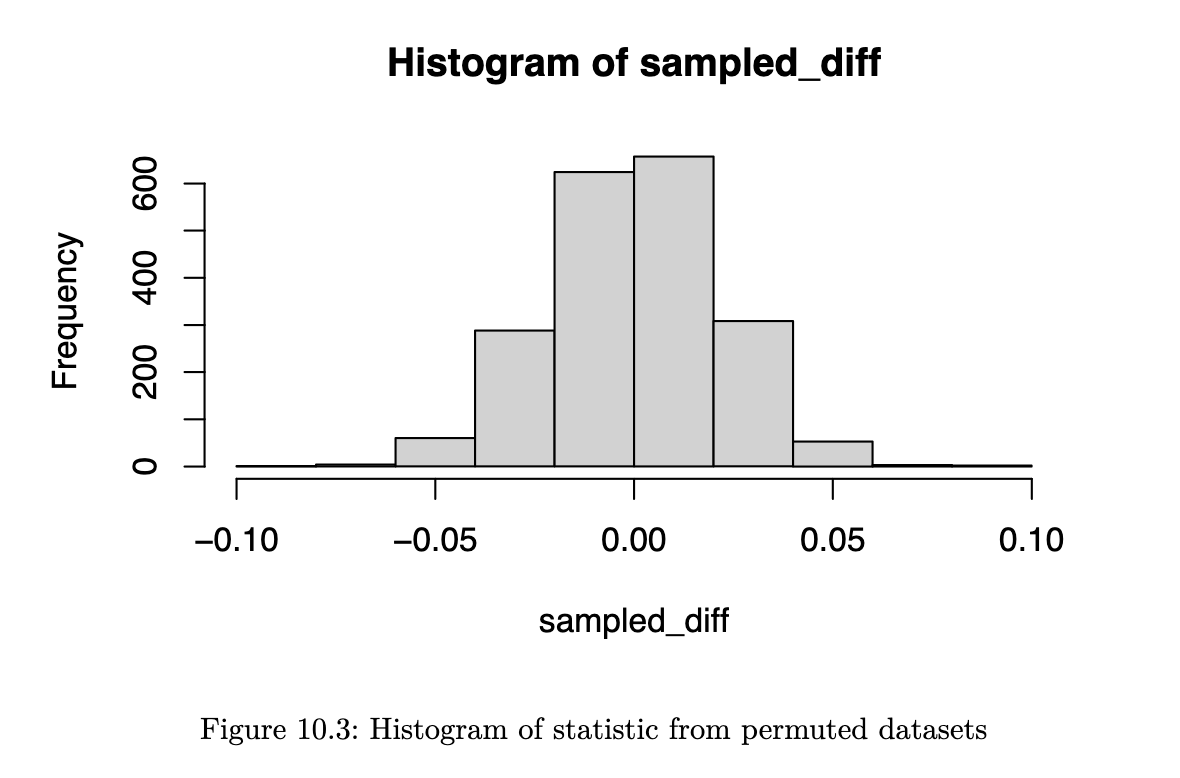

(p_val <- 2*mean(sampled_diff > d1))
 
# [1] 0.369

Bootstrapping

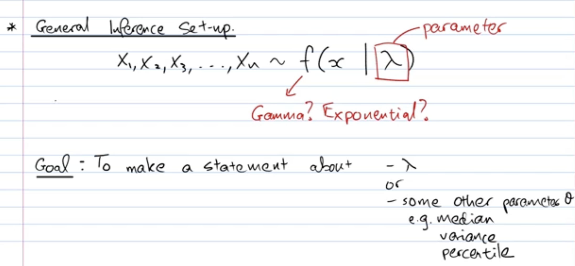
The bootstrap procedure is a general purpose tool for understanding the variability in estimators for which we do not know the distribution. In standard inference techniques, we aim to find out more about a “population”, using a dataset “sample”-d from it.

The ingenious idea behind the bootstrap is this:

The uncertainty that arises from using the sample data to infer about the population, is analogous to the uncertainty that arises when using bootstrap samples to infer about the original sample.

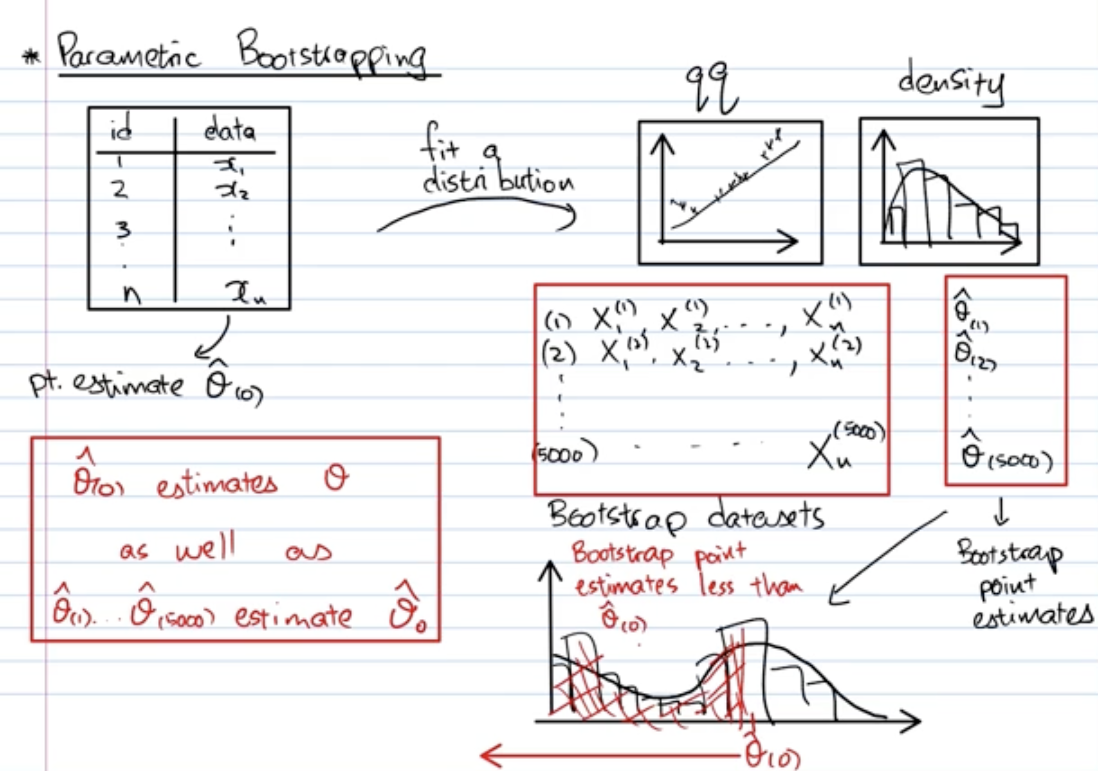
One of the greatest benefits of the bootstrap is the ability to provide confidence intervals for estimators for which we may not know how to derive analytic or asymptotic results.

1. More accurate intervals
2. No need to assume Normality

Consider obtaining a confidence interval for the trimmed mean, that we encountered in L5 Robust Statistics.

Example 10.9

library(MASS)
 
mean(chem)
 
# [1] 4.280417
 
t.test(chem)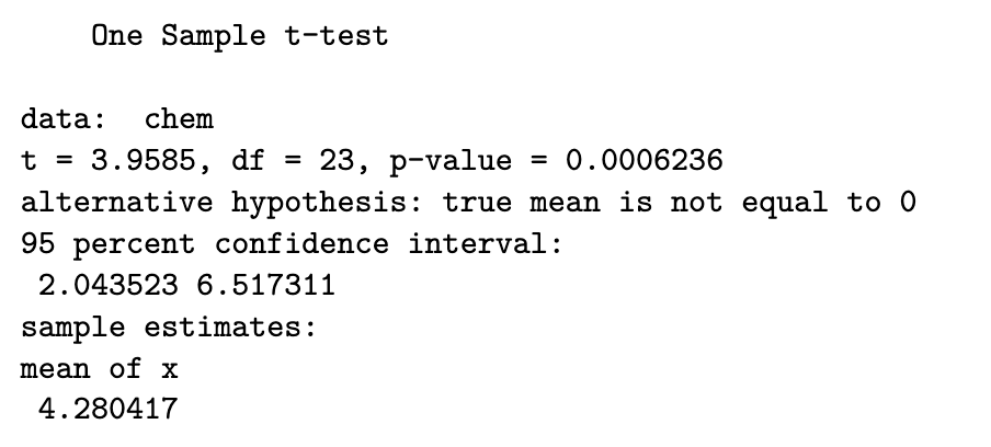

Notice how the CI from the non-robust technique is very wide.

library(boot)
 
stat_fn <- function(d, i) {
  b <- mean(d[i], trim=0.1)
  b
}
boot_out <- boot(chem, stat_fn, R = 1999, stype="i")
# Returns two types of bootstrap intervals:
boot.ci(boot.out = boot_out, type=c("perc", "bca"))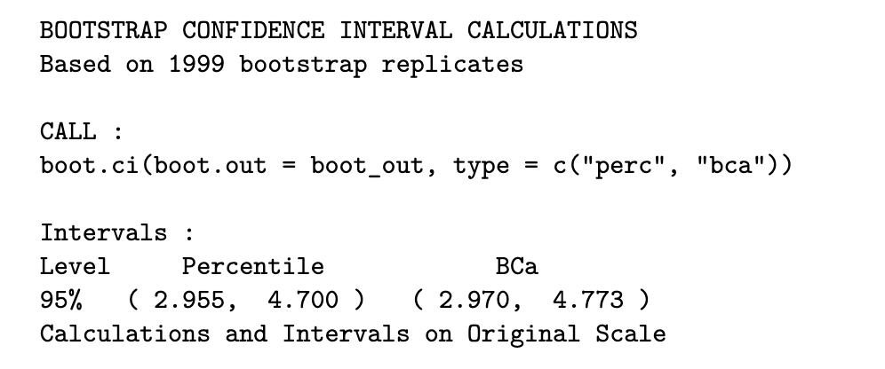

The boot function requires a function (stat_fn) that computes the statistic from the boot-strapped sample. Note that the intervals returned from the trimmed mean are much narrower. Moreover, from Example 5.5, we know that the trimmed mean for the chem dataset is 3.205. Hence the above output shows that the bootstrap intervals are asymmetric, reflecting the skewness of the distribution of the statistic.

stuff not in lec notes:

uniroot(f, interval, ...) — Root Finding in R

Finds where a function f crosses zero within interval = c(lo, hi).

# Find where g2(lambda) = 0, i.e. where the pdf equals a given ordinate
r1 <- uniroot(g2, c(0.00001, 1.27), y=y_vals, alpha=alpha, beta=beta,
              ordinate=ordinate)$root

• f must change sign across the interval (one positive end, one negative end)
• returns a list; extract the root with $root
• extra named arguments (e.g. ordinate=) are passed through to f

---

Vectorize(f, vectorize.args) — Vectorise a Scalar Function

Wraps a function so it accepts vector inputs element-wise (analogous to numpy.vectorize).

g3 <- Vectorize(g3, "ordinate")   # now g3(c(0.1, 0.5, 0.9)) works

Needed when passing a function to uniroot that is not naturally vectorised.

---

Summary

For our course, please be familiar with the basic building blocks of simulation studies:

1. Generate iid samples, and then
2. Compute the sample mean, and the CI for the true mean.