L7 Two-sample Hypothesis Tests

Introduction

In this topic, we introduce the routines for a common class of hypothesis tests: the scenario of comparing the location parameter of two groups. This technique is commonly used in A/B testing to assess if an intervention has resulted in a significant difference between two groups.

Hypothesis tests are routinely abused in many ways by investigators. Such tests typically require strong assumptions to hold, and can result in false positives or negatives. As such, it may be preferred to use confidence intervals to make an assessment of the significance of a result. In this topic, we introduce how the p-values can be obtained for these hypothesis tests.

Procedure for Significance Tests

Step 1: Assumptions

In this step, we verify that the assumptions required for the test are valid. In some tests, this step is carried out at the end of the others, but it is always essential to perform. Some tests are very sensitive to the assumptions - this is the main reason that the class of Robust Statistics was invented.

Step 2: State the hypotheses and significance level

The purpose of hypothesis testing is to make an inferential statement about the population from which the data arose. This inferential statement is what we refer to as the hypothesis regarding the population.

NOTE:
A hypothesis is a statement about population, usually claiming that a parameter takes a particular numerical value or falls in a certain range of values.

The hypothesis will be stated as a pair: The null hypothesis H0 and the alternative hypothesis H1. Both statements will involve the population parameter (not the data summary) of interest.

For example, if we have a sample of observations from two groups A and B and we wish to assess if the mean of the populations is different, the hypotheses would be:

$$H_0:{\mu }_A={\mu }_B$$ $$H_1:{\mu }_A\ne {\mu }_B$$

H0 is usually a statement that indicates “no difference”, and H1 is usually the complement of H0.

At this stage, it is also crucial to state the significance level of the test. The significance level corresponds to the Type I error of the test - the probability of rejecting H0 when in fact it was true. This level is usually denoted as 𝛼, and is usually taken to be 5%, but there is no reason to adopt this blindly. Think of the choice of 5% as corresponding to accepting an error rate of 1 in 20 - that’s how it was originally decided upon by Fisher.

WARNING:
It is important to state the significance level at this stage because if it is chosen after inspecting the data, the test is no longer valid. This is because, after knowing the p-value, one could always choose the significance level such that it yields the desired decision.

Example of one-tailed test:

$$H_0:{\mu }_A={\mu }_B$$ $$H_1:{\mu }_A>{\mu }_B$$

Step 3: Compute the Test Statistic

The test statistic is usually a measure of how far the observed data deviates from the scenario defined by H0. Usually, the larger it is, the more evidence we have against H0.

The construction of a hypothesis test involves the derivation of the exact or approximate distribution of the test statistic under H0. Deviations under the assumption could render this distribution incorrect.

Step 4: Compute the p-value

The p-value quantifies the chance of observing such a test statistic, or one that is more extreme in the direction of H1, under H0. The distribution of the test statistic under H0 is used to compute this value between 0 and 1. A value closer to 0 indicates stronger evidence against H0.

Step 5: State your conclusion

If the p-value is less than the stated significance level, we conclude that we reject H0. Otherwise, we say that we do not reject H0. It is conventional to use this terminology (instead of saying “accept H1”) since our p-value is obtained with respect to H0.

Confidence Intervals

Confidence intervals are an alternative method of inference for population parameters. Instead of yielding a binary reject / do-not-reject result, they return a confidence interval that contains the plausible values for the population parameter. Many confidence intervals are derived by inverting hypothesis tests, and almost all confidence intervals are of the form:

$$\text{Sample estimate}\pm \text{margin of error}$$

For instance, if we observe x1, … , xn from a Normal distribution, and wish to estimate the mean of the distribution, the 95% confidence interval based on the t distribution is

$$\bar{x}\pm t_{0.025,n-1}\times \frac{s}{\sqrt{n}}$$

where:

• s is the sample standard deviation, and
• t_0.025,n-1 is the 0.025-quantile from the t distribution with n-1 degrees of freedom

The formulae for many confidence intervals rely on asymptotic Normality of the estimator. However, this is an assumption that can be overcome with the technique of bootstrapping Bootstrapping.

Bootstrapping can also be used to sidestep the distributional assumptions in hypothesis tests, but the professor prefers confidence intervals to tests because they yield an interval, providing much more information than a binary outcome.

Parametric Tests

Parametric tests are hypothesis tests that assume some form of distribution for the sample (or population) to follow. An example of such a test is the t-test, which assumes that the data originates from a Normal distribution.

Conversely, nonparametric tests are hypothesis tests that do not assume any form of distribution for the sample. Unfortunately, since nonparametric tests are so general, they do not have a high discriminative ability - they have low power. In other words, if a dataset truly comes from a Normal distribution, using the t-test would be able to detect smaller differences between the groups better than a non-parametric test.

In this section, we cover parametric tests for comparing the difference in mean between two groups.

Independent Samples Test

In an independent samples t-test, observations in one group yield no information about the observations in the other group. Independent samples can arise in a few ways:

• in an experimental study, study units could be assigned randomly to different treatments, thus forming the two groups
• in an observational study, we could draw a random sample from the population, and then record an explanatory categorical variable on each unit, such as the gender or senior-citizen status
• in an observational study, we could draw a random sample from a group (say smokers), and then a random sample from another group (say non-smokers). This would result in a situation where the independent 2-sample t-test is appropriate

Formal Set-up

Formally speaking, this is how the independent 2-sample t-test works:
Suppose that X1, X2, … , Xn are independent observations from group 1, and Y1, … Yn2 are independent observations from group 2. It is assumed that:

$$\begin{array}{rl}{X}_i& \sim N({\mu }_1,{\sigma }^2),i=1,\dots ,n_1\\ Y_j& \sim N({\mu }_2,{\sigma }^2),j=1,\dots ,n_2\end{array}\text{\hspace{1em}(7.1)(7.2)}$$

The null and alternative hypotheses would be:

$$\begin{array}{r}{H}_0:{\mu }_1={\mu }_2\\ H_1:{\mu }_1\ne {\mu }_2\end{array}$$

The test statistic for this test is:

$$T_1=\frac{(\bar{X}-\bar{Y})-0}{s_p\sqrt{1/n_1+1/n_2}}$$

where

$$s_p^2=\frac{(n_1-1)s_1^2+(n_2-1)s_2^2}{n_1+n_2-2}$$

Under $H_0$, the test statistic $T_1\sim t_{n_1+n_2-2}$. When we use a software to apply the test above, it will typically also return a confidence interval, computed as

$$(\bar{X}-\bar{Y})\pm t_{n_1+n_2-2,1-\alpha /2}\times s_p\sqrt{1/n_1+1/n_2}$$

The set-up above corresponds to the case where the variance within each group is assumed to be the same. We use information from both groups to estimate the common variance. If we find evidence in the data to the contrary, we use the unpooled variance in the denominator of $T_1$ :

$$T_{1,unpooled}=\frac{(\bar{X}-\bar{Y})-0}{\sqrt{s_1^2/n_1+s_2^2/n_2}}$$

where $s_1^{2}and{s}_2^2$ are the sample variance from groups 1 and 2. The test statistic still follows a t distribution, but the degrees of freedom are approximated. This approximation is known as the Satterthwaite approximation.

Example 7.1 (Abalone Measurements)

The dataset contains measurements of physical characteristics, along with the gender status. We derive a sample of 50 measurements of male and female abalone records for use here. Our goal is to study if there is a significant difference between the viscera weight between males and females.

R code

abl <- read.csv("data/abalone_sub.csv")
x <- abl$viscera[abl$gender == "M"]
y <- abl$viscera[abl$gender == "F"]
 
t.test(x, y, var.equal=TRUE)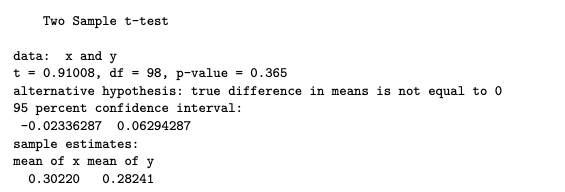

import pandas as pd
import numpy as np
from scipy import stats
import statsmodels.api as sm
 
abl = pd.read_csv("data/abalone_sub.csv")
#abl.head()
#abalone_df.describe()
 
x = abl.viscera[abl.gender == "M"]
y = abl.viscera[abl.gender == "F"]
 
t_out = stats.ttest_ind(x, y)
ci_95 = t_out.confidence_interval()
 
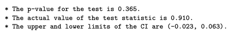
print(f"""
* The p-value for the test is {t_out.pvalue:.3f}.
* The actual value of the test statistic is {t_out.statistic:.3f}.
* The upper and lower limits of the CI are ({ci_95[0]:.3f}, {ci_95[1]:.3f}).
""")

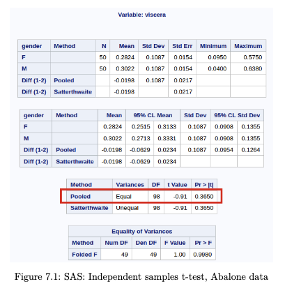
SAS Output

The assumptions of the test include Normality and equal variance. Let us assess the equality of variance first. While there are many hypothesis tests specifically for assessing if variances are equal (eg. Levene, Bartlett), the prof has a simple rule of thumb in this class:

if the larger sd is more than twice the smaller one, then we should not use the equal variance form of the tests

• use the above to assess homogeneity of variances (empirical rule)

# EXAMPLE
# Assess homogeneity of variances (empirical rule)  
 
group_sds <- tapply(taiwan2$price, taiwan2$num_stores, sd)  
  
max_sd <- max(group_sds)  
min_sd <- min(group_sds)  
  
ratio <- max_sd / min_sd  
ratio

R code

aggregate(viscera ~ gender, data=abl, sd)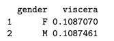

Python code

abl.groupby('gender').describe()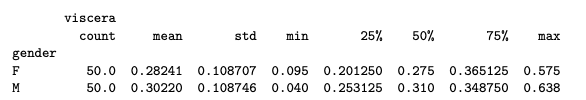

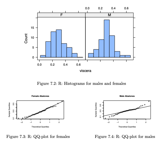
To assess the Normality assumption, we make histograms and qq-plots.
(See Histograms and QQ-plots)

library(lattice)
histogram(~viscera | gender, data=abl, type="count")
qqnorm(y, main="Female Abalones"); qqline(y)
qqnorm(x, main="Male Abalones"); qqline(x)

We would conclude that there is no significant difference between the mean viscera weight of males and females.

Apart from qq-plots, it is worthwhile to touch on additional methods that are used to assess how much a dataset deviates from Normality.

More on Assessing Normality

Skewness

The Normal distribution is symmetric about its mean. Hence if we observe asymmetry in our histogram, we might suspect deviation from Normality. To quantify this asymmetry, we use skewness. One method of estimating skewness of a distribution from data is:

$$g_1=\frac{\frac{1}{n}{\sum }_{i=1}^n(x_i-\bar{x}{)}^3}{{\left(\frac{1}{n}{\sum }_{i=1}^n(x_i-\bar{x}{)}^2\right)}^{3/2}}$$

This is the method-of-moments estimator for the distribution skewness parameter. A value close to 0 indicates low skewness (ie. high symmetry). Positive values correspond to right-skew and negative values to left-skew.

Kurtosis

Kurtosis measures the thickness of the tails of a distribution. Positive kurtosis implies that the tails are “fatter” than those of a Normal. Negative values indicate that the tails are “thinner” than those of a Normal.

The method of moments estimator is:

$$g_2=\frac{\frac{1}{n}{\sum }_{i=1}^n(x_i-\bar{x}{)}^4}{{\left(\frac{1}{n}{\sum }_{i=1}^n(x_i-\bar{x}{)}^2\right)}^2}-3$$

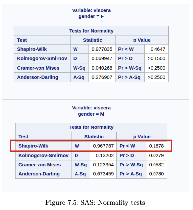
Hypothesis tests for Normality

The Shapiro-Wilk test and the Kolmogorov-Smirnov test are formal hypothesis tests with the following hypotheses:

$$\begin{array}{rl}{H}_0& :\text{Data follows a normal distribution}\\ H_1& :\text{Data does not follow a normal distribution}\end{array}$$

Take note that applying multiple tests leads to a higher Type I error (false positive). Moreover, a large sample size will almost always reject $H_0$ because small deviations are being classified as significant. The prof advocates a more graphical approach in assessing Normality, especially since the solution to Non-normality (the bootstrap) is readily accessible today.

Example 7.2 (Abalone Measurements)

R code

library(DescTools)
aggregate(viscera ~ gender, data=abl, Skew, method=1)
## gender viscera
## 1 F 0.4060918
## 2 M 0.2482997
 
aggregate(viscera ~ gender, data=abl, Kurt, method=1)
## gender viscera
## 1 F -0.2431501
## 2 M 1.1660593
 
# Shapiro-Wilk Test only for males:
shapiro.test(x)
##
## Shapiro-Wilk normality test
##
## data: x
## W = 0.96779, p-value = 0.1878

Python code

abl.groupby("gender").skew()
## viscera
## gender
## F 0.418761
## M 0.256046
 
for i,df in abl.groupby('gender'):
print(f"{df.gender.iloc[0]}: {df.viscera.kurt():.4f}")
## F: -0.1390
## M: 1.4220
 
stats.shapiro(x)
## ShapiroResult(statistic=np.float64(0.9677872659314101), pvalue=np.float64(0.1878490793650714

SAS output

Although the skewness seems large for the female group, the Normality tests do not reject the null hypothesis.

Paired Sample test

The data in a paired sample test also arises from two groups, but the two groups are not independent. A very common scenario that gives rise to this test is when the same subject receives both treatments. His / her measurement under each treatment gives rise to a measurement in each group. However, the measurements are no longer independent.

Example 7.3 (Reaction time of drivers)

Study of 32 drivers sampled from a driving school. Whenever the driver sees red, he/she has to press a brake button. For each driver, the study is carried out twice. Each measurement falls under “phone” or “radio”, but the measurements for driver i are clearly related. Some people might just have a slower / faster baseline reaction time. This is a situation where a paired sample test is appropriate, not an independent sample test.

Formal Set-up

Suppose that we observe $X_1,\dots ,X_n$ independent observations from group 1 and $Y_1,\dots ,Y_n$ independent observations from group 2. However, the pair $(X_i,Y_i)$ are correlated. It is assumed that

$$\begin{array}{r}{X}_i\sim N({\mu }_1,{\sigma }_1^2),i=1,\dots ,n\\ Y_j\sim N({\mu }_2,{\sigma }_2^2),j=1,\dots ,n\end{array}\text{\hspace{1em}(7.3)(7.4)}$$

We let $D_i=X_i-Y_i$ for i = 1,…,n. It follows that

$$D_i\sim N({\mu }_1-{\mu }_2,{\sigma }_1^2+{\sigma }_2^2-2cov(X_i,Y_i))$$

The null and alternative hypotheses are stated in terms of the distribution of $D_i$ :

$$\begin{array}{r}{H}_0:{\mu }_D=0\\ H_1:{\mu }_D\ne 0\end{array}$$

The test statistic for this test is:

$$T_2=\frac{\bar{D}-0}{s/\sqrt{n}}$$

where

$$s^2=\frac{{\sum }_{i=1}^n(D_i-\bar{D}{)}^2}{(n-1)}$$

Under $H_0$, the test statistic $T_2\sim t_{n-1}$. When we use a software to apply the test above, it will typically also return a confidence interval, computed as

$$\bar{D}\pm t_{n-1,1-\alpha /2}\times s/\sqrt{n}$$

Example 7.4 (Heart Rate Before / After Treadmill)

R code

To run the paired test, we run the same function t.test as earlier, but we set the argument paired.

hr_df <- read.csv("data/health_promo_hr.csv")
before <- hr_df$baseline
after <- hr_df$after5
t.test(before, after, paired=TRUE)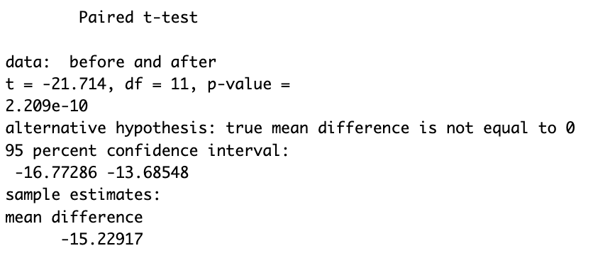

Python code

hr_df = pd.read_csv("data/health_promo_hr.csv")
#hr_df.head()
 
paired_out = stats.ttest_rel(hr_df.baseline, hr_df.after5)
print(f"""
Test statistic: {paired_out.statistic:.3f}.
p-val: {paired_out.pvalue:.3f}.""")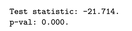

SAS Output

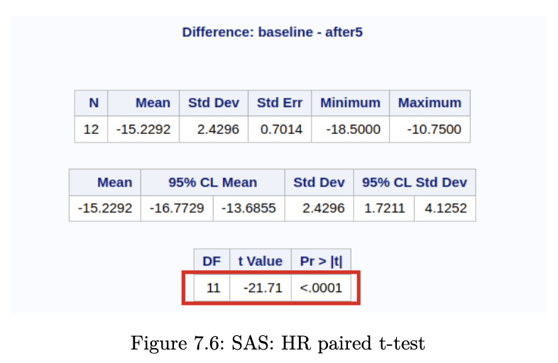
It is imperative to also make the checks for Normality. If you were to make them, you would realise that the sample size is rather small - it is difficult to make the case for Normality here.

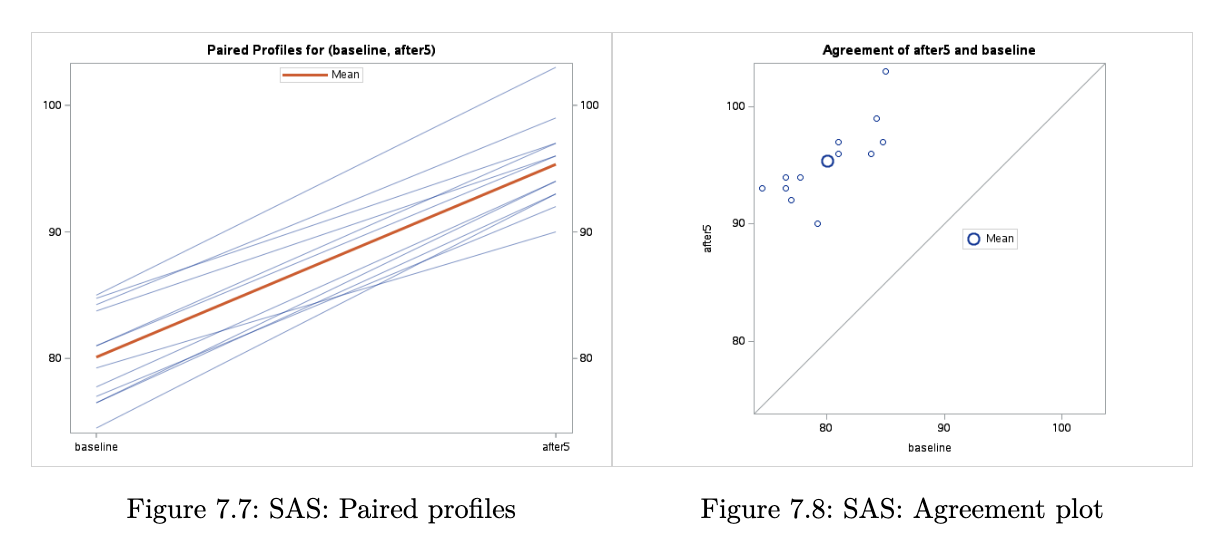
When we inspect the paired plot, we are looking for a similar gradient for each line, or at least similar in sign. If instead, we observed a combination of positive and negative gradients, then we would be less confident that there is a difference in means between the groups.

For the agreement plot, if we were to observe the points scattered around the line y = x, then we would be more inclined to believe that the mean difference is indeed 0.

Non-parametric Tests

If the distributional assumptions of the t-test are not met, we can take action in several ways. Historically, one method was to transform the data (if it was skewed) to make the histogram symmetric and thus closer to a Normal. But this was not ideal - it did not help in cases where the data was symmetric but had fatter tails than the Normal.

As time progressed, tools were invented to overcome the distributional assumptions.

• one sub-field was Robust Statistics, which keep the assumptions to a minimum eg. only requiring the underlying distribution to be symmetric
• another sub-field was the area of non-parametric statistics, where almost no distributional assumptions were made about the data.

In this section, we cover the non-parametric analogues for independent and paired 2-sample tests.

Independent Samples Test

The non-parametric analogue of the independent 2-sample test is the Wilcoxon Rank Sum (WRS) Test (equivalent to the Mann-Whitney test)

Formal Set-up

Suppose that we observe $X_1,\dots ,X_{n_1}$ independent observations from group 1 (with distribution F) and $Y_1,\dots ,Y_{n_2}$ independent observations from group 2 (with distribution G).
The hypotheses associated with this test are:

$$\begin{array}{l}{H}_0:F=G\\ H_1:F(x)=G(x-\Delta ),\Delta \ne 0\end{array}$$

In other words, the alternative hypothesis is that the distribution of group 1 is a location shift of the distribution of group 2.

The WRS test begins by pooling the $n_1+n_2$ data points and ranking them. The smallest observation is awarded rank 1, and the largest observation is awarded rank $n_1+n_2$, assuming there are no tied values. If there are tied the values, the observations with the same value receive an average rank.

Compute $R_1$, the sum of the ranks in group 1. If this sum is large, it means that most of the values in group 1 were larger than those in group 2. Note that the average rank in the combined sample is

$$\frac{n_1+n_2+1}{2}$$

Under $H_0$, the expected rank sum of group 1 is

$$E(R_1)=n_1\times \frac{n_1+n_2+1}{2}$$

The test statistic is a comparison of $R_1$ with the above expected value:

$$W_1=\{\begin{array}{ll}\frac{\left|R_1-\frac{n_1(n_1+n_2+1)}{2}\right|-\frac{1}{2}}{\sqrt{n_1{n}_2(n_1+n_2+1)/12}}& R_1\ne \frac{n_1(n_1+n_2+1)}{2}\text{ and no ties}\\ \frac{\left|R_1-\frac{n_1(n_1+n_2+1)}{2}\right|-\frac{1}{2}}{\sqrt{n_1{n}_2\left((n_1+n_2+1)-\frac{{\sum }_{i=1}^g{t}_i(t_i^2-1)}{(n_1+n_2)(n_1+n_2-1)}\right)/12}}& R_1\ne \frac{n_1(n_1+n_2+1)}{2}\text{ and ties present}\\ 0& R_1=\frac{n_1(n_1+n_2+1)}{2}\end{array}$$

where g refers to the number of groups with ties, and $t_i$ refers to the number of tied values in each group.

The test above should only be used if both $n_1$ and $n_2$ are at least 10, and if the observations (not the ranks) come from an underlying continuous distribution. If these assumptions hold, then the test statistic $W_1$ follows a $N(0,1)$ distribution.

Example 7.5 (Abalone Measurements)

R code

We can perform the WRS test in R:

wilcox.test(x,y)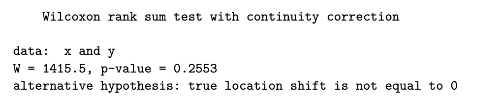

Python code

As mentioned, the Mann-Whitney test will return the same p-value as the WRS test.

wrs_out = stats.mannwhitneyu(x,y) 
 
print(f"""Test statistic: {wrs_out.statistic:.3f}.
p-val: {wrs_out.pvalue:.3f}.""")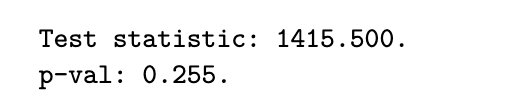

SAS Output

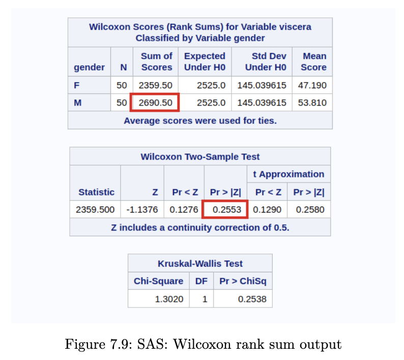
Since we know the number of observations in each group to be more than 10, the approximation holds. Comparing with Example 7.1 (Abalone Measurements), we observe that we have a similar conclusion.

Notice that the test statistic appears different in SAS. However, it is simply a matter of a location shift of the test statistic. R and python subtract the smallest possible sum of ranks from group 1, but SAS does not. In our example, the group size is 50. Hence we can recover the SAS test statistic from the R test statistic with

$$1415.5+\frac{50(50+1)}{2}=2690.5$$

The p-value is identical in all three software.

Paired Samples Test

The analogue of the paired sample t-test is known as the Wilcoxon Sign Test (WST)

Formal Set-up

Again, suppose that we observe $X_1,\dots ,X_n$ observations from group 1 and $Y_1,...,Y_n$ observations from group 2. Groups 1 and 2 are paired (or correlated in some way).
Once again, we compute $D_i=X_i-Y_i$ . The null hypothesis is that

$$\begin{array}{l}{H}_0:\text{median of }{D}_i\text{ is 0.}\\ H_1:\text{median of }{D}_i\text{ is not 0.}\end{array}$$

We begin by ranking the $|D_i|$. Ignoring pairs for which $D_i=0$, we rank the remaining observations from 1 for the pair with the smallest absolute value, up to n for the pair with the largest absolute value (assuming no ties).

We then compute $R_2$, the sum of ranks for the positive $D_i$. If this sum is large, we expect that the pairs with $X_i>Y_i$ have a larger difference (in absolute values) than those with $X_i<Y_i$ . Under $H_0$, it can be shown that

$$E(R_2)=m(m+1)/4$$

where m is the number of non-zero differences.

Thus the test statistic is a comparison of $R_2$ with the above expected value:

$$W_2=\{\begin{array}{ll}\frac{\left|R_2-\frac{n(n+1)}{4}\right|-\frac{1}{2}}{\sqrt{n(n+1)(2n+1)/24}}& \text{if }{R}_2\ne \frac{n(n+1)}{4}\text{ and no ties}\\ \frac{\left|R_2-\frac{n(n+1)}{4}\right|-\frac{1}{2}}{\sqrt{n(n+1)(2n+1)/\left(24-\frac{{\sum }_{i=1}^g(t_i^3-t_i)}{48}\right)}}& \text{if }{R}_2\ne \frac{n(n+1)}{4}\text{ and ties present}\\ 0& \text{if }{R}_2=\frac{n(n+1)}{4}\end{array}$$

where g denotes the number of tied groups, and $t_i$ refers to the number of differences with the same absolute value in the i-th tied group.

If the number of non-zero $D_i$‘s is at least 16, then the statistic $W_2$ follows a $N(0,1)$ distribution approximately.

Example 7.6 (Heart Rate Before / After Treadmill)

R code

wilcox.test(before, after, paired=TRUE, exact=FALSE)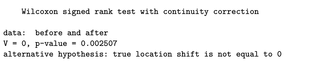

Python code

wsr_out = stats.wilcoxon(hr_df.baseline, hr_df.after5, 
						correction=True, method='approx')
 
print(f"""Test statistic: {wsr_out.statistic:.3f}.
p-val: {wsr_out.pvalue:.3f}.""")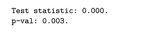

SAS Output

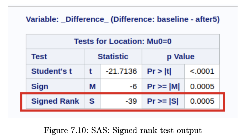
In this problem, we do not have 16 non-zero $D_i$‘s. Hence we should in fact be using the “exact” version of the test (R and Python). However, the exact version of the test cannot be used when there are ties.

SAS does indeed use the “exact” version of the test, so that accounts for the difference in p-values. The test statistic in SAS is computed by subtracting $E(R_2)$, but in R and Python this subtraction is not done. To get from test statistic in R (0) to the one in SAS (-39):

$$0-\frac{12(12+1)}{4}=-39$$

In cases like these, we can turn to the bootstrap, or we can use a permutation test.