L5 Robust Statistics

Introductory statistics courses describe and discuss inferential methods based on the assumption that data is Normally distributed. However, the sample itself may deviate from Normality in various ways. (eg. heavy tails, skew)

Another way in which the Normal-based method could breakdown is when our dataset has extreme values, referred to as outliers. In such cases, many investigators will drop the anomalous points and proceed with the analysis on the remaining observations. This is not ideal for the following reasons:

1. the sharp decision to reject an observation is wasteful. we can do better by down-weighting the dubious observations
2. it can be difficult to spot or detect outliers in multivariate data

Continuing to use Normal based methods will result in confidence intervals and hypothesis tests that have low power. Instead, statisticians have developed a suite of methods that are robust to the assumption of Normality. These techniques may be sub-optimal when the data is truly Normal, but they quickly outperform the Normal-based method as soon as the distribution starts to deviate from Normality.

Notation

$$\text{Suppose we have an i.i.d. sample }{X}_i\text{ from a continuous pdf }f,\text{ where }i=1,\dots ,n.$$ $$\text{1. We use }{q}_{f,p}\text{ to refer to the p-th quantile of f, i.e.}$$ $$P(X\le q_{f,p})=p$$ $$\text{2. For standard Normal quantiles, we use }{z}_p$$ $$\varphi (z_p)=P(Z\le z_p)=p$$ $$\text{3. We denote the order statistics from the sample with }{X}_{(i)}.\text{ In other words,}$$ $$X_{(1)}\le X_{(2)}\le \dots \le X_{(n)}$$ $$\text{We denote the sample median as }{X}_{(1/2)}.$$

Datasets

For this topic, we are working with a couple of datasets that are clearly not Normal.

Copper in Wholemeal Flour Dataset (Chem)

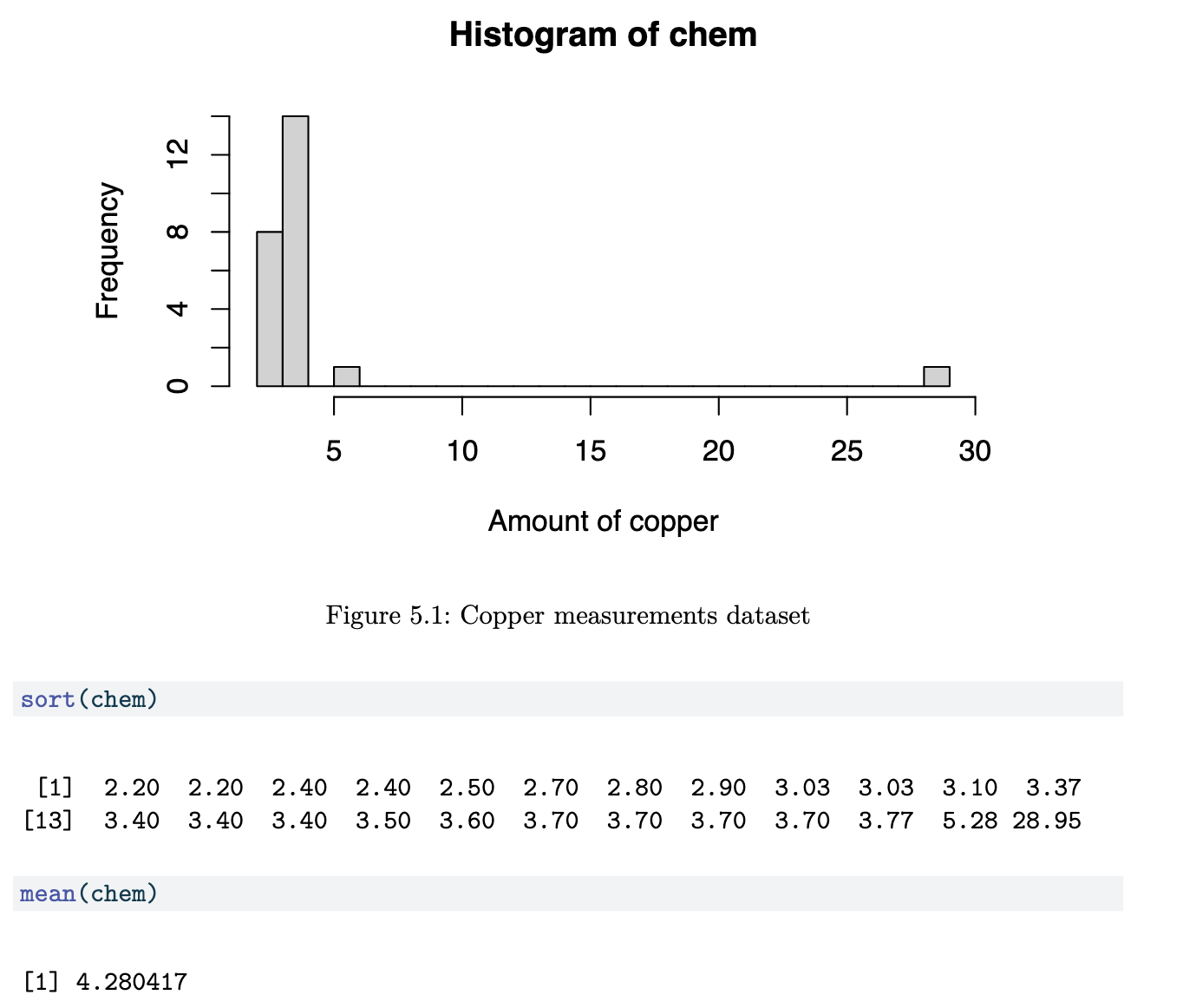
Although 22 of the 24 points are less than 4, the mean is 4.28. This statistic is clearly being affected by the largest two values. This topic is about techniques that will work well even in the presence of such large anomalous values.

Self-Awareness Dataset

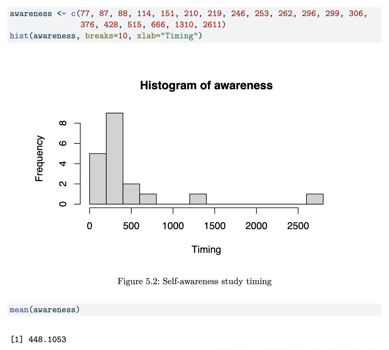
Just like the data in the first example, this data is too highly skewed to the right. The mean of the full dataset is larger than the 3rd quartile.

Assessing Robustness

Asymptotic Relative Efficiency

Suppose we wish to estimate a parameter 𝜃 of a distribution using a sample of size n.

$$\text{We have two candidate estimators }\hat{\theta }\text{ and }\tilde{\theta }.$$

Definition 5.1: Asymptotic Relative Efficiency (ARE).

$$\text{The ARE of }\tilde{\theta }\text{ relative to }\hat{\theta }\text{ is}$$ $$ARE(\tilde{\theta };\hat{\theta })=\underset{n\to \infty }{\lim }\frac{varianceof\hat{\theta }}{varianceof\tilde{\theta }}$$

Usually, 𝜃^ is the optimal estimator according to some criteria. The intuitive interpretation is that when using 𝜃^, we only need ARE times as many observations as when using 𝜃~. Smaller values of ARE indicate that 𝜃^ is better than 𝜃~.

Here are a couple of commonly used estimators and their AREs.

Example 5.4 (Contaminated Normal Variance Estimate)

Suppose that we have n observations, Yi ~ N(𝜇, 𝜎2) and we wish to estimate 𝜎2. Consider the two estimators:

$$1.{\hat{\sigma }}^2=s^2=\frac{1}{n-1}\sum _{i=1}^n(Y_i-\bar{Y}{)}^2$$ $$2.{\tilde{\sigma }}^2=d^2\pi /2,\text{ where}$$ $$d=\frac{1}{n}\sum _i|Y_i-\bar{Y}|$$

In this case, when the underlying distribution truly is Normal, we have

$$ARE({\tilde{\sigma }}^2;{\hat{\sigma }}^2)=87.6\%$$

However, now consider a situation where Yi ~ N(𝜇, 𝜎2) with probability 1 - 𝜖 and Yi ~ N(𝜇, 9𝜎2) with probability 𝜖. Let us refer to this as a contaminated Normal distribution.

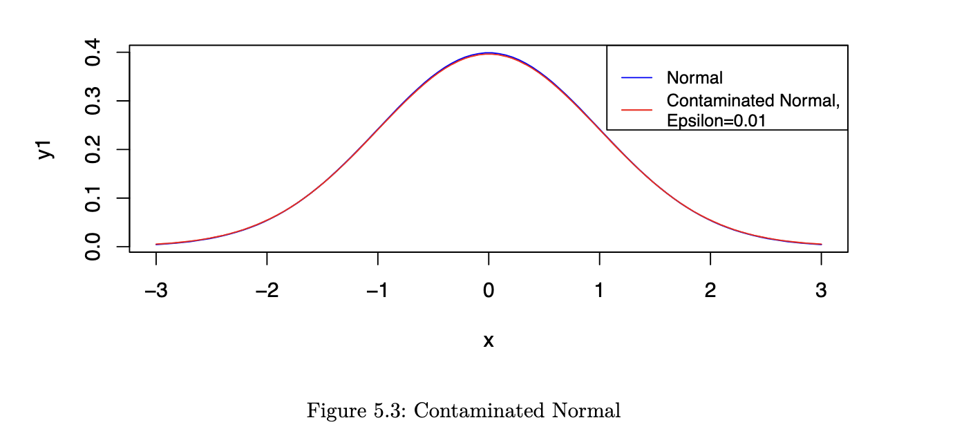
As you can see from the figure, the two pdfs are almost indistinguishable by eye. However, the ARE values are very different:

𝜖      ARE
-------------
0      87.6%
0.01   144%

The usual s^2 loses optimality very quickly; we can obtain more precise estimates using 𝜎~ ^2.

Requirements of Robust Summaries

1. Qualitative Robustness
   • if the underlying distribution F changes slightly, then the estimate should not change too much.
2. Infinitesimal Robustness
   • this is tied to the concept of the influence function of an estimator.
   • roughly speaking, the influence function measures the relative extent that a small perturbation in F has on the value of the estimate.
   • in other words, it reflects the influence of adding one more observation to a large sample
3. Quantitative Robustness
   • this is related to the contaminated distribution we touched on in example 5.4. consider:

$$F_{x,ϵ}=(1-ϵ)F+ϵ{\Delta }_x$$

- where Δ𝑥 is the degenerate probability distribution at x. 
- the minimum value of 𝜖 for which the estimator goes to infinity as x gets large, is referred to as the **breakdown point**. 
- for the sample mean, the breakdown point is 𝜖 = 0.5

Measures of Location

The location parameter of a distribution is a value that characterises a “typical” observation, or the middle of the distribution. It is not always the mean of the distribution, but in the case of a symmetric distribution it will be.

1. M-estimators

Before we introduce robust estimators for the location, let us revisit the most commonly used one - the sample mean. Suppose we have observed x1,x2…xn, a random sample from a 𝑁(𝜇, 𝜎2) distribution. As a reminder, here is how we derive the MEL for 𝜇.

The likelihood function is

$$L(\mu ,{\sigma }^2)=\prod _{i=1}^n\frac{1}{\sqrt{2\pi {\sigma }^2}}{e}^{-(x_i-\mu {)}^2/2{\sigma }^2}$$

(equation 5.1) The log-likelihood is

$$\log L=l(\mu ,{\sigma }^2)=-n\log (\sigma )-\frac{n}{2}\log (2\pi )-\frac{1}{2{\sigma }^2}\sum _{i=1}^n(x_i-\mu {)}^2$$

Setting the partial derivative with respect to 𝜇 to be 0, we can solve for the MLE:

$$\frac{\partial l}{\partial \mu }=0$$ $$\frac{1}{{\sigma }^2}\sum _{i=1}^n(x_i-\hat{\mu })=0$$ $$\hat{\mu }=\bar{x}$$

Observe that in equation 5.1, we minimised the sum of squared errors, which arose from minimising

$$\sum _{i=1}^n-\log f(x_i-\mu )$$

where f is the standard normal pdf. Instead of using log f, Huber proposed using alternative functions (let’s call the function 𝜌 (rho)) to derive estimators. The new estimator corresponds to: (equation 5.2)

$$\arg \underset{\mu }{\min }\sum _{i=1}^n\rho (x_i-\mu )$$

The choice of 𝜌 confers certain properties on the resulting estimator. For instance, 𝜓 = 𝜌’ is referred to as the influence function, which measures the relative change in a statistic as a new observation is added. To find the 𝜇^ that minimises equation 5.2, it is equivalent to setting the derivative to zero and solving for 𝜇^:

$$\sum _{i=1}^n\psi (x_i-\mu )=0$$

Note that, in general, the use of the sample mean corresponds to the use of 𝜌(x) = x^2. In that case, 𝜓 = 2x is unbounded, which results in high importance / weight placed on very large values. Instead, robust estimators should have a bounded 𝜓 function.

The approach outlined above - the use of 𝜌 and 𝜓 to define estimators, gave rise to a class of estimators known as M-estimators, since they are MLE-like. In the following sections, we shall introduce estimators corresponding to various choices of 𝜌. It is not always easy to identify the 𝜌 being used, but inspection of the form of 𝜓 leads to an understanding of how much emphasis the estimator places on large outlying values.

2. Trimmed mean

The 𝛾-trimmed mean (0 < 𝛾 ⇐ 0.5) is the mean of a distribution after the distribution has been truncated at the 𝛾 and 1-𝛾 quantiles. Note that the truncated function has to be renormalised in order to be a pdf.

In formal terms, suppose that X is a continuous random variable with pdf f. The usual mean is of course just 𝜇 = ∫ 𝑥𝑓(𝑥)𝑑𝑥. The trimmed mean of the distribution is: (equation 5.3)

$${\mu }_t={\int }_{q_{f,\gamma }}^{q_{f,1-\gamma }}x\frac{f(x)}{1-2\gamma }dx$$

Using the trimmed mean focuses on the middle portion of a distribution. The recommended value of 𝛾 is (0, 0.2]. For a sample X1, X2, … Xn, the estimate is computed using the following algorithm:

1. compute the value 𝑔 = ⌊𝛾𝑛⌋, where ⌊𝑥⌋ refers to the floor function
   • floor function: the largest integer less than or equal to x
2. drop the largest g and smallest g values from the sample
3. compute

$${\hat{\mu }}_t=X_t=\frac{X_{(g+1)}+\dots X_{(n-g)}}{n-2g}$$

It can be shown that the influence function for the trimmed mean is

$$\psi (x)=\{\begin{array}{ll}x,& -c<x<c\\ 0,& \text{otherwise}\end{array}$$

which indicates that, with this estimator, large outliers have no effect on the estimator.

3. Winsorised Mean

The Winsorised mean is similar to the trimmed mean in the sense that it modifies the tail of the distribution. However, it works by replacing extreme observations with fixed moderate values. The corresponding 𝜓 function is

$$\psi (x)=\{\begin{array}{ll}-c,& x<-c\\ x,& |x|<c\\ c,& x>c\end{array}$$

Just like in the trimmed mean case, we decide on the value c by choosing a value 𝛾 ∈ (0, 0.2]. To calculate the Winsorised mean from a sample X1,X2,…,Xn, we use the following algorithm:

1. compute the value 𝑔 = ⌊𝛾𝑛⌋
2. replace the smallest g values in the sample with X_(g+1) and the largest g values with X_(n-g)
3. compute the arithmetic mean of the resulting n values

$$X_w=\frac{g\cdot X_{(g+1)}+X_{g+1}+\cdots +X_{n-g}+g\cdot X_{(n-g)}}{n}$$

Important! Note that the trimmed mean and the Winsorised mean are no longer estimating the population distribution mean 𝑥𝑓(𝑥)𝑑𝑥. The three quantities coincide only if the population distribution is symmetric. When this is not the case, it is important to be aware of what we are estimating. For instance, using the trimmed / winsorised mean is appropriate if we are interested in what a “typical” observation in the middle of the distribution looks like.

Measures of Scale

1. Sample Standard Deviation

Just as in the M-Estimators section, the MLE of the population variance 𝜎2 is not robust to outliers. It is given by

$$s^2=\frac{1}{n}\sum _{i=1}^n(x_i-\bar{x}{)}^2$$

Here are a few robust alternatives to this estimator. However, take note that, just like in the case of location estimators, the following estimators are not estimating the standard deviation. We can modify them so that if the underlying distribution truly is Normal, then they do estimate 𝜎. However, if the distribution is not Normal, we should treat them as they are: robust measures of the spread of the distribution.

2. Median Absolute Deviation

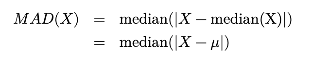
For a random variable X ~ f, the median absolute deviation w is defined by

$$P(|X-q_{f,0.5}|\le w)=0.5$$

We sometimes refer to w as MAD(X). In other words, it is the median of the distribution associated with |X - q_f,0.5|; it is the median of absolute deviations from the median.

If observations are truly from a Normal distribution, it can be shown that MAD estimates 𝑧_0.75𝜎. Hence, in general, MAD is divided by 𝑧_0.75 so that it coincides with 𝜎 if the underlying distribution is Normal.

Proposition 5.1 (MAD for Normal).

$$ForX\sim N(\mu ,{\sigma }^2),\text{ the following property holds:}$$ $$\sigma \approx 1.4826\times MAD(X)$$

Proof. Note that, since the distribution is symmetric, median(X) = 𝜇. Thus,

Thus, the MAD(X) is a value q such that

$$P(|X-\mu |\le q)=0.5$$

Equivalently, we need q such that

$$P\left(\left|\frac{X-\mu }{\sigma }\right|\le \frac{q}{\sigma }\right)=P\left(|Z|\le \frac{q}{\sigma }\right)=0.5$$

Remember that we can retrieve values for the standard Normal cdf easily from R or Python:

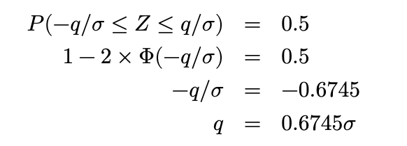
Thus MAD(X) = 0.6745𝜎. The implication is that we can estimate 𝜎 in a standard Normal with

$$\hat{\sigma }\approx \frac{1}{0.6745}MAD(X)$$

3. Interquartile Range

The general definition of IQR(X) is

$$q_{f,0.75}-q_{f,0.25}$$

It is a linear combination of quantiles. Again, we can modify the IQR so that, if the underlying distribution is Normal, we are estimating the standard deviation 𝜎.

Proposition 5.2 (IQR for Normal). For X ~ N(𝜇, 𝜎2), the following property holds:

$$\sigma \approx \frac{IQR(X)}{1.35}$$

Proof. For X ~ 𝑁 (𝜇, 𝜎2), let q_0.25 and q_0.75 represent the 1st and 3rd quartiles of the distribution.

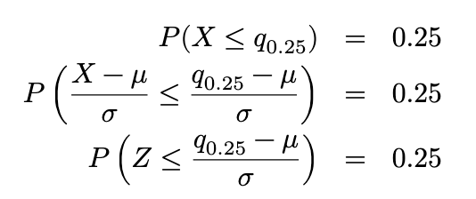
Thus (from R or Python) ((in R: qnorm(0.25))), we know that

$$\frac{q_{0.25}-\mu }{\sigma }=z_{0.25}=-0.6745$$ $$\therefore q_{0.25}=\mu -0.6745\sigma$$

Similarly, we can derive that q_0.75 = 𝜇 + 0.6745𝜎. Now we can derive that

$$IQR(X)=q_{0.75}-q_{0.25}\approx 1.35\sigma$$

The implication is that, if we have sample data from standard Normal, we can estimate 𝜎 from the IQR using:

$$\hat{\sigma }=\frac{IQR(\{X_1,\dots ,X_n\})}{1.35}$$

Examples

Example 5.5

(location estimates: copper dataset)

R code

mean(chem) 
## [1] 4.280417
 
mean(chem, trim=0.1) # using gamma = 0.1
## [1] 3.205
 
library(DescTools)
vals <- quantile(chem, probs=c(0.1,0.9))
win_sample <- Winsorize(chem,vals) # gamma = 0.1
mean(win_sample) 
## [1] 3.182375

import pandas as pd
import numpy as np 
from scipy import stats 
 
chem = pd.read_csv("data/mass_chem.csv")
 
chem.chem.mean() 
## np.float64(4.2804166666666665)
 
stats.trim_mean(chem, proportiontocut=0.1)
## array([3.205])
 
stats.mstats.winsorize(chem.chem, limits=0.1).mean()
## np.float64(3.185)

As we observe, the robust estimates are less affected by the extreme and isolate value 28.95. They are more indicative of the general set of observations

Example 5.6

(scale estimates: copper dataset)

R code

sd(awareness)
## [1] 594.6295
 
mad(awareness, constant=1)
## [1] 114 
 
IQR(awareness) 
## [1] 221.5

awareness = np.array([77, 87, 88, 114, 151, 210, 219, 246, 253, 262, 296,
	299, 306, 376, 428, 515, 666, 1310, 2611])
	
awareness.std() 
## np.float64(578.7698292373723)
 
stats.median_abs_deviation(awareness) 
## np.float64(114.0)
 
stats.iqr(awareness)
## np.float64(221.5)